Geodetic Adjustment Australia

THE GEODETIC ADJUSTMENT OF AUSTRALIA, 1963-1966

(originally in the SURVEY REVIEW No. 144, 1967, Vol. XIX)

A. G. Bomford

National Mapping, Canberra

ABSTRACT

The geodetic surveys in Australia were adjusted on the new Australian Geodetic Datum in 1966. There is now a homogeneous series of co-ordinates for all geodetic stations in Australia, New Guinea and the islands in. the Bismarck Sea, on which future mapping and a grid reference system will be based. This paper describes the method of adjustment.

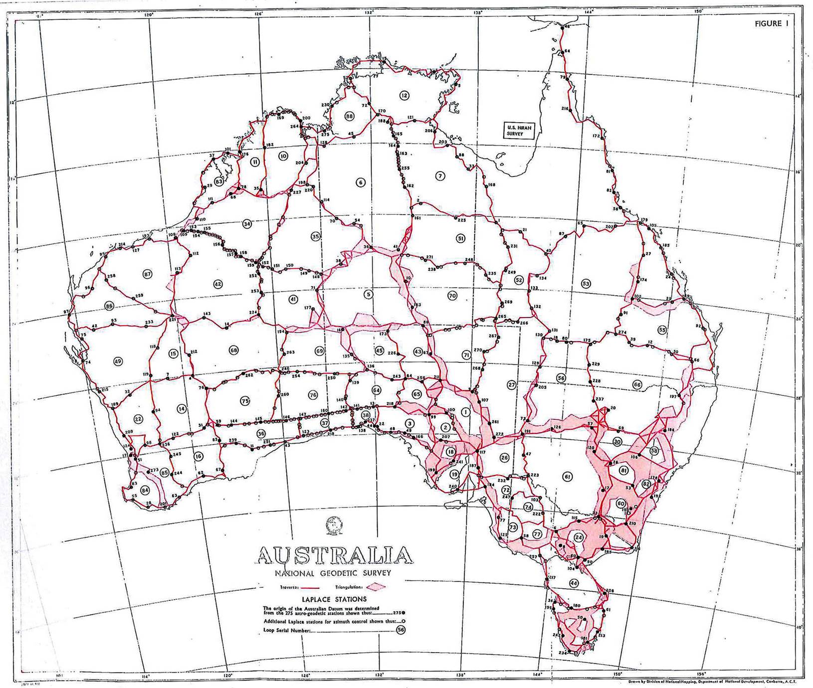
The geodetic survey of Australia at the close of the 1965 field season is shown in Figure 1. There are 2506 stations of which 533 are Laplace stations. In addition to the geodetic triangulation, there are 33,100 miles of tellurometer traverse. This work was computed and adjusted on the new Australian Geodetic Datum during the first half of 1966. This paper describes the methods used. Parts of this paper were included in an interim paper to the Ninth Australian Survey Congress (1966a), when the work was still in progress. Work prior to June 1963 has previously been described (1963a).

COMPUTING MACHINERY

In June 1964, the Commonwealth Scientific and Industrial Research Organisation installed a Control Data Corporation 3600 computer in Canberra. National Mapping had jobs ready to run on this machine the day it was installed, and have used it daily ever since. It is a powerful machine, capable of 100,000 additions and 100,000 floating-point multiplications in one second; a word consists of ten floating-point decimal digits, very suitable for surveyors; and the high-speed store holds 32,000 words. Programs can be written in an advanced version of Fortran, which is compiled into machine-language at about the speed of the card reader, 800 cards per minute, with very detailed diagnostic information when errors are detected. Provided the theory of what is to be done is well understood, programs are easy to write, and cheap to test and revise. It is a rare day when the machine is not working, and the fault then generally lies with the air-conditioning system. Although now two years old, and thus out of date by current, standards of computer technology, it will long remain a wonderful machine.

COMPUTER PROGRAMS

The survey programs previously in use have been rewritten, benefiting from several years experience on smaller machines. The CDC 3600 is so fast that it is possible to incorporate every desirable refinement at a cost of only fractions of seconds in running time. New and more ambitious programs have been written. The most powerful, and most used, is a program for the least squares adjustment of surveys by the method of variation of co-ordinates on the spheroid (1966b). This program will adjust any combination of angles, azimuths and distances between 100 variable and 40 fixed points. There is no limit to the number of observations. The formulae used are accurate to less than one inch at 1000 miles, so that Aerodist and Hiran lines may be included in an adjustment. Much of this program was written before the computer was installed, and it first ran in September 1964, though additions are still made. Over 140 different networks have been adjusted, most of them many times.

The input consists of rounds of directions taken from the field-book or abstract, Laplace azimuths, and measured distances. Approximate latitude and longitudes have also to be listed. This is sometimes a little inconvenient with Aerodist surveys, when the initial positions of the stations may have to be read from a small-scale map, and the adjustment iterated two or three times. But the compensating advantages of the variation of co-ordinates method are great as no conditions have to be listed; and the adjusted latitudes and longitudes are produced immediately, as well as the adjusted angles, azimuths and distances, without further computation. It is the sum of the weighted squares of the adjustments to the observations which is minimised, not the adjustments to the latitudes and longitudes. The adjustment is by the method of angles. Both G. Bomford (1962, p. 101) and Rainsford (1957, p. 73) recommend the adjustment of angles rather than directions, even if the angles have been observed in rounds. The matter is still being discussed (Allman and Bennett, 1966), but unless the adjustment of directions is known to be definitely the better, the adjustment of angles will usually be preferred for variation of co-ordinates. The number of unknowns is simply two per station, whereas the adjustment of directions requires either an extra unknown for each station, or the complexity of Schreiber's device for eliminating it (Rainsford, 1957, p. 175).

The subroutine for the solution of the normal equations was written by Mr. R. H. Hudson, of the CSIRO Computing Research Section, Canberra. It is based on the method of Cholesky, but makes use of the fact that in most survey adjustments the non-zero coefficients in the normal equations can be made to lie in a band adjacent to the principal diagonal. The zeros outside the band are not stored. This reduces the number of multiplications required in the solution, and since a matrix of order 200 and band-width 60 contains only 10,370 elements, the whole solution can be carried out in the high-speed store. Direct methods have been criticised for use in electronic computers, on the grounds that if the equations are ill-conditioned, round-off errors may accumulate and make the solution worthless. In survey networks, a strong fix for all the stations is one of the surveyor's chief aims, so the equations should never be seriously ill-conditioned; and in practice, Cholesky's method has been found entirely satisfactory. It is nevertheless a wise precaution to prove that all is well by iterating every adjustment at least once.

Computation is very quick. From reading the first card of data to printing the last line of output, the following times are typical :-

1. The Ridgeway Base Figure (Rainsford, 1962, p. 364) containing 7 stations, 19 angles and 14 distances: 14.6 seconds, the solution of the normal equations taking 0.16 seconds.

2. The geodetic survey of Tasmania, with 94 variable points, 385 angles, 9 azimuths and 102 distances: 5 minutes 7 seconds, the solution of the normals taking 2 minutes 47 seconds.

Numerous options and refinements are available. The program usually works with normal section azimuths, but geodesic azimuths can be used if preferred. Changes in Laplace azimuths due to the adjustment in longitude of the observation stations are automatically allowed for. If the input is in feet, the output can be in metres. Transverse Mercator co-ordinates of the adjusted points can be included in the output, using Redfearn's (1948) formulae in full. The closing angle of a round is usually included as an observation, but may be excluded if desired. In addition to the adjusted quantities, the adjustments and the observed quantities are normally printed out, but may be suppressed. The average and maximum adjustments of each type are normally printed for each station and for the complete adjustment. Provided there is a redundancy available, the program draws attention to errors in the data which are significantly larger than the random errors of observation. Each observation may be individually weighted, and a variety of general weighting systems are available.

WEIGHTING SYSTEMS

It still seems to be a controversial question whether weights are dimensioned quantities or not, but the question can be avoided. If we ignore any correlation between the observed quantities, then it is beyond dispute that in any least squares adjustment, but particularly one which contains mixed units such as angles and distances, each observation equation must be divided by the standard error of the observed quantity or by some number bearing a constant proportion to it. In this context it is immaterial whether we consider standard errors or probable errors. Both are dimensioned quantities. On dividing through, all the observation equations become dimensionless. Provided the observations are uncorrelated, and provided the standard errors we have used are in the correct ratio to each other, the method of least squares then gives us the most probable adjustments to the observed quantities.

If we do not divide each observation equation by the standard error of the observed quantity, that is, if we ignore weights, we are tacitly assuming that the standard errors of our angles and distances are in the ratio of one second to one foot, or one second to one metre; we obtain a different adjustment according to the units we use. For the long lines common in geodetic work, if distances are expressed in feet, the resulting adjustments may not be unsatisfactory, When the program was first written, weights were not used, and with remarkable regularity the average adjustment to a direction was about 0.3 seconds and to a tellurometer distance about 0.3 feet, with maxima of about 1".3 and 1.3 feet. When distances were expressed in metres, the adjustments to distances were almost doubled. The author sometimes wonders if the suspicion in which the tellurometer was long held in some countries was not in part due to ignoring weights in least squares adjustments, expressing distances in metres, and thus forcing adjustments into distances which should have properly been applied to angles. If distances were customarily expressed in millimetres or kilometres the effect would be more dramatic. An essential test of any least squares computer program is to run a test job twice, with distances in different units, and confirm that identical results are obtained.

The second weighting system built into the program was that suggested by Murphy (1958). This system gives effect to the belief that at the end of a line whose length and azimuth have both been measured, the error ellipse is circular, with its radius proportional to the length of the line, L. This is achieved by dividing observation equations for distances by (L sin 1"). The system depends for its efficacy on the fact that Wadley, in designing the tellurometer, produced an instrument whose accuracy closely matches that of a geodetic theodolite. If the standard error of a distance is say 3.5 parts per million then the Murphy system allocates a standard error to a direction of 0".7, which is not unreasonable. But with short distances, adjustments tend to zero, and with telluormeter distances, this is certainly wrong: there is always a residual uncertainty of about 0.1 feet however short the line; and Laplace azimuths, which have a different standard error to directions, must be individually weighted. This system is now only used for adjustments containing both tellurometer lines and short accurately taped distances.

The third weighting system introduced was a modification of the Murphy system, designed for continental adjustments, where each "observation" consists of the length or azimuth of a complete section of survey. If errors in tellurometer distances and Laplace azimuths are random, then the error in the length or azimuth of a section should be proportional to the square root of its length. So the error ellipse, whilst still assumed to be circular, was given a radius proportional to the square root of the length of the section. This was achieved by dividing observation equations for distances, and multiplying observation equations for azimuths, by (L sin 1")^½. This system is not used for adjustments containing observed angles. Besides continental adjustments, it has also been used for Hiran and Aerodist adjustments.

The fourth weighting system introduced, and the one now in standard use, is based on a priori standard errors, expressed in seconds of arc for directions and for azimuths, and as the vector sum of a fixed distance plus so many parts per million for distances. For the final computations of the 1966 geodetic adjustment of Australia, the following standard errors were used:

Angles: 0".7, or directions 0".5. This is equivalent to an average triangle closure of 1".0. Much of the triangulation in Australia has smaller average triangle closures; but on traverses there is not the same continual check on the quality of the work, and some of the angular work may be less good. Directions observed on fewer than 20 zeros, and all second-order observations, were individually under-weighted. No directions were over-weighted, no matter how many zeros had been observed. An unusually large number of zeros usually indicates that observations were proving troublesome.

Laplace Azimuths: A standard error of 1".0 for a single-ended observation. The mean misclosure of 120 reciprocal Laplace azimuths was 1".18, equivalent to a standard error of 1".0 for the observations at one end. Reciprocal azimuths were meaned, and inserted from one end of the line only, with double weight. If the reciprocal azimuth observations were simultaneous, as was generally the case, they were given treble weight, on the grounds that refraction errors tend to cancel in the mean. The internal standard error of the astronomic azimuths and longitudes was generally about 0".2, and skilled observers may think that the adopted standard error of 1".0 is too high. But angles and azimuths were observed on a similar number of zeros; angles can be observed during the optimum conditions of twilight, whereas azimuths to Sigma Octantis cannot be observed till after dark; level errors are greater to elevated stars; and Laplace azimuths are additionally burdened by the error in the astronomic longitude. If angles have a standard error of 0".7, the standard errors of 1".0 for a single-ended Laplace azimuth, and 0".45 for an azimuth derived from simultaneous reciprocal observations, seem reasonable. Any survey organisation still observing Laplace azimuths from only one end of a line, and believing it is getting azimuths with standard errors of about 0".2, should observe a few pairs of reciprocal azimuths. The results are always interesting, often chastening.

Tellurometer Distances: A standard error equal to the vector sum of 0.1 feet plus 3 parts per million. This is a well established value. The few distances measured with the Model 1 geodimeter were given double weight.

The various weighting systems have been compared on four typical sections of triangulation in New South Wales and Victoria. The average adjustments obtained are shown in Table 1.

TABLE 1

Average adjustments obtained with different weighting systems, in four sections of geodetic triangulation in Victoria and N.S.W. The sections contain a total of 794 angles, 15 azimuths and 130 distances.

	Directions (seconds)	Azimuths	Distances (feet)
Weighting system
Free adjustments:
No weights
Distances in feet	0.30	0.35	0.24
Distances in metres	0.28	0.32	0.48 (ft)
Murphy	0.33	0.36	0.18
A priori standard errors	0.33	0.53	0.17

Forced adjustments:
A priori standard errors	0.35	0.38	0.21

THE AUSTRALIAN NATIONAL SPHEROID

Until April 1965, the "165 " spheroid was in use :

a = 6,378,165metres; 1/f = 298.3.

This spheroid has been superseded. It was hoped that a new international spheroid might be universally adopted, but so far no agreement has been reached by surveyors. Numerous modern spheroids are in use overseas, with the radius in the range 6,378,148 to 6,378,169 metres, and the flattening in the range of 298.2 to 298.3. These spheroids do not differ significantly one from another, and it is a pity that international agreement has not been reached. It would be convenient for satellite geodesy, and a single set of tables could be prepared for those who still have occasion to compute by hand.

The International Astronomical Union (Fricke, 1965) have, however, agreed on a spheroid for astronomical use :

a = 6,378,160 metres; l/f = 298.25.

Though not specifically intended for geodetic use, this is as good a spheroid as any other. It has at least some international backing, and the National Mapping Council adopted it for the Australian National Spheroid in April 1965.

THE JOHNSTON ORIGIN

The "Central Origin" in use since 1963 was based on 155 astro-geodetic stations distributed over most of Australia with the exception of Cape York and Tasmania. Since then, about 100 Laplace stations have been observed each year, and by December 1965 the total number in Australia was 533 - see Figure 1. From these, 275 stations were selected on the following principles:-

1. The distribution over the whole of Australia (including Cape York and Tasmania, but excluding New Guinea) should be as uniform as possible.

2. Where two stations lie close together, a station whose longitude was observed with an impersonal micrometer on a T4 or DKM3a theodolite should be preferred to a station observed with a fixed-wire eyepiece on a geodetic theodolite.

No corrections for the topography were applied. On the Australian National Spheroid and the Central Origin, the mean deflection at these 275 stations was :

+0".15 in meridian; -0".36 in prime vertical.

The question arose whether these values were large enough to warrant a change of origin. In March 1965, 224 stations were analysed by splitting Australia into quarters, and finding the mean deflection in each quarter :

	Meridian	Prime Vertical	No. of Stations
NE	+0".17	-1.02	39
SE	+0 .67	-0.17	67
SW	+0 .08	+0.02	57
NW	-1 .40	-0.24	61
Weighted Mean	-0 .02	-0.29	Total 224

In February 1966 a similar analysis was made of 142 stations which were located in flat areas :

	Meridian	Prime Vertical	No. of Stations
NE	-1".61	-0.90	21
SE	+1 .08	+0.34	40
SW	+0 .67	-0.88	43
NW	-0 .89	-0.94	39
Weighted Mean	+0 .03	-0.56	Total 142

It is evident that random undulations in the geoid make it impossible to locate a centre for the spheroid with a standard error of less than 0".5, about 15 metres, even with a very large number of stations. (Analyses of satellite orbits, supported by the Tranet satellite observations and the 1966 results from the Baker-Nunn cameras, suggest that there is probably a fairly uniform tilt in the geoid across Australia, a rise of about 90 metres from south-west to north-east, which cannot be detected by astro-geodetic observations within Australia itself. For a picture, see Veis, 1965, p. 40. This tilt corresponds to deflections of about 4" in meridian and 3' in prime vertical and implies that the centre of the Australian National Spheroid may be as much as 160 metres from the earth's centre of gravity).

The Central Origin was therefore retained, but it is now defined in terms of the Johnston Memorial Cairn. The Central Origin was originally defined in terms of the trigonometrical station Grundy, whose spheroidal height, for lack of any information to the contrary, was taken equal to its geoidal height :

S: 25° 54' 11". 078; E: 134° 32' 46". 457; Height: 1304 feet.

The equivalent values for the Johnston Memorial Cairn are :

S: 25° 56' 54". 5515; E 133° 12' 30". 0771; Height: 571.2 metres.

These values for the Johnston Origin locate the centre of the spheroid with reference to the mark beneath the Johnston Memorial Cairn. The spheroid is oriented by defining the minor axis to be parallel to the earth's mean axis of rotation at the start of 1962, (Parallel with respect to the solid earth. With respect to the stars, both the earth and its axis change direction due to precession and notation) and by defining the origin of geodetic longitude to be 149° 00' 18".855 west of the vertical through the photo zenith tube at Mount Stromlo (in other words, " Greenwich", the Australian component of the BIH mean observatory. The size, shape, position and orientation of the spheroid are thus completely defined, and together define the Australian Geodetic Datum. At the conclusion of the 1966 National Adjustment, the mean deflection on the Australian Geodetic Datum of the 275 selected stations was:

+ 0" .12 in meridian; -0" .33 in prime vertical.

THE METHOD OF ADJUSTMENT

The geodetic survey of Australia was divided into 161 sections between 101 junction points, forming 58 loops - see Figure 1. Using the variation of coordinates program, each section was first freely adjusted, holding only one point fixed. From these free adjustments, the azimuths and distances between the junction points were obtained by Robbins's (1962) formulae. Using the variation of co-ordinates program, the azimuths and distances between the junction points were put into a single adjustment covering the mainland of Australia, and final co-ordinates for the junction points obtained. Each section was then readjusted holding the co-ordinates of the junction points fixed.

Tasmania was connected to the mainland by two additional sections across Bass Strait, one via King Island, one via Flinders Island. The tellurometer traverse up Cape York, together with the United States Air Force Hiran network (1965) and the geodetic survey of New Guinea, gave co-ordinates on the Australian Geodetic Datum for a further 135 stations in New Guinea and the Bismarck Archipelago.

HEIGHTS

Perhaps the greatest weakness in the geodetic survey is the absence of a continental height adjustment. The various authorities had to adjust misclosures in height in whatever manner seemed expedient. Discrepancies exist at junction points, and in some areas the heights now in use may prove to be in error by 20 feet or more. Twenty feet is equivalent to one part per million in the distances. Yet there would be little value in obtaining better heights above the geoid while the separation of the geoid and the spheroid remains unknown. Apart from a local survey at Woomera (1963b), no geoidal sections have been observed in Australia, and there may well be a separation between the geoid and the spheroid of the order of 20 feet anywhere in the continent. (If the geoidal tilt across Australia suggested by satellites really exists, it will not introduce correspondingly large errors into our distances. A more or less uniform geoid slope will have affected all the astro-geodetic stations used to determine the Johnston Origin, causing a corresponding displacement of the spheroid). It is intended to start some transcontinental geoidal sections in 1967. A National Levelling Adjustment is scheduled for 1970, to which all triangulation and traverse heights will be adjusted. An improved national adjustment may be run, for scientific purposes only, in 1971 or 1972.

Heights for each station were tabulated in the data for the variation of co-ordinates program, and were listed in the output; but they played no direct part in the adjustment. Care was taken to ensure that the heights tabulated were those used for the reduction of the tellurometer distances. If better heights became available, the tellurometer distances were changed accordingly, though the change in any individual distance was usually trivial.

DISTANCES

All measured distances were tabulated in International Feet:

1 International Foot = 0.3048 metres exactly.

The chord-to-arc correction used by all authorities, except the New South Wales Lands Department, was L³/24R². Distances were therefore modified by a small computer program to change the chord-to-arc correction to L³/24R², a value which allows for the curvature of the radio path and its dip into regions of greater refractive index. On long lines, the effect was remarkable. In New Guinea two tellurometer measurements of about 120 miles had been rejected, as they required adjustments of 6.5 and 10.6 feet. The change in the chord-to-are correction was over 9 feet, and both lines are now acceptable. A third line of 120 miles has since been measured and required an adjustment of less than one foot.

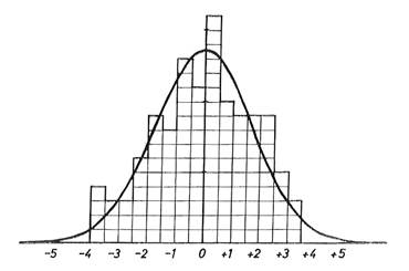
Figure 2. Closures of 59 loops in latitude and longitude, in parts
per million of the loop length. Average closure 1.38 ppm.
Normal distribution with σ = 1.73 superimposed.

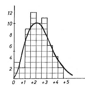
Figure 3. Vector loop closures of 59 loops as parts

per million of the loop length. Average closure 2.19 ppm.

Normal two-dimensional distribution with

σ = 1.73 in each dimension superimposed.

THE FREE ADJUSTMENTS

The aim of the free adjustments was to find the most probable values for the azimuths and distances between the junction points. Whenever convenient, smaller sections were combined, and the 161 sections were fitted into 114 separate adjustments. Overlaps beyond the junction points were not unusual: any observation which could significantly affect the azimuth and distance between one junction point and its neighbour was included. Normal section azimuths were used. Extreme care was taken to see that the Laplace azimuths were in terms of the preliminary longitudes, and the program then maintained this relationship automatically. With a traverse, the free adjustment merely adjusted the angles and the Laplace azimuths, leaving the distances unchanged, and took only a few seconds. The largest adjustment contained 76 points, with 383 angles, 9 azimuths and 50 distances, and kept the computer busy for 3½ minutes.

After every run, the output was very carefully inspected. A least-squares adjustment of a modern tellurometer traverse running through old triangulation is a severe test of any authority's methods and records, and the program contains so many traps for imperfect data that it sometimes seemed remarkable that any adjustment ran at all. The diagnostic information provided by the program made it easy to locate errors. As soon as a reasonable adjustment was obtained, the second or third run the average and maximum adjustments had generally been reduced to values which experience suggested were satisfactory. Any adjustment exceeding 1".5 in a direction or an azimuth or 1.5 feet in a distance was investigated.

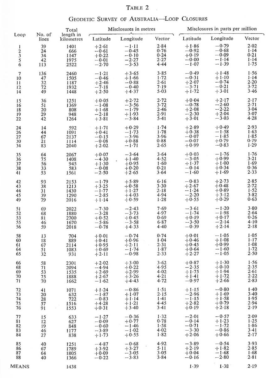
Whenever a number of sections forming a loop had been adjusted satisfactorily, the loop closure in latitude and longitude was computed. Each loop was given a serial number - see Figure 1. The closures are tabulated in Table 2, and shown in Figures 2 and 3. As the original large loops were gradually subdivided, it was to be expected that the closures, expressed as parts per million of the loop length, would tend to increase: errors had less chance to randomise out. The average loop length is now about 900 miles, and the average closure 2.2 parts per million, with a maximum of 4.3. The few small loops without loop numbers were included within single adjustments.

THE INVERSE COMPUTATIONS

When a section appeared satisfactory, and the loop closure confirmed that all was well, the geodesic azimuth and distance between its junction points was determined from their adjusted latitudes and longitudes. The formulae used in the computer were those given by Robbins (1962). Tests of this program over the ACIC (1959) test lines have confirmed that Robbins's formulae are highly accurate at distances up to 1000 miles. Normal section azimuths are exact, and in the worst case the error in distances was 2 cm. Using formula (3.8) in Geodesy (G. Bomford, 1962) to obtain geodesic azimuths from normal section azimuths gave a worst error of 0".06 at 1000 miles.

THE NATIONAL ADJUSTMENT

The geodesic azimuths and distances between neighbouring junction points were put into a single least-squares adjustment covering the mainland of Australia, using the same variation of co-ordinates program. Azimuths and distances were weighted inversely as the length of each section. Care was taken to see that the preliminary longitudes of the junction points were those used in the computation of the azimuths, so that the Laplace conditions remained undisturbed. The co-ordinates of the trigonometrical station Grundy in the centre of Australia were held fixed, and adjusted latitudes and longitudes for all other junction points were obtained. The first trial adjustment of this type was run on 21 June 1965, using the 140 sections then available.

In this adjustment it was still assumed that the error ellipse at the end of a section was circular, but there is good evidence to show that this is not true. Since nearly all the sections have a tellurometer traverse running through them, their variation in linear accuracy in parts per million is not great. In contrast, their accuracy in azimuth varies greatly. Some sections are chains of triangulation; others are traverses. Some have only a single-ended azimuth every eight stations; others have reciprocal azimuths on every line.

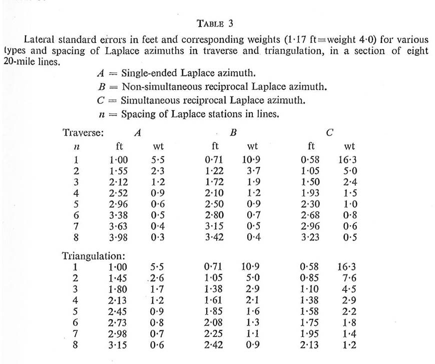
A section of eight traverse lines each 20 miles long was taken as a model. The linear standard error at the end of the section was calculated assuming a constant error in each line of 0.1 foot, plus a random error of 3 parts per million:

[(8 x 0.1)²+ (8^½ x 0.3)²]^½ = 1.17 feet.

For the lateral standard error, the contributions from the angles and the
azimuths were first considered separately. For the angles, formula (16) on page 598
of Jordan (1950) was used :

If l is the length of a line, here taken as 20 miles,

n is the number of stations in the traverse, and

s is the standard error of a traverse angle, here taken as 0" .5 x √(2) = 0".7,

then the lateral standard error due to the angles is approximately

This was calculated for n = 5 (four lines) and n = 9 (eight lines), with l = 20 miles.

This formula applies to a traverse. A triangulation chain can be loosely considered as a combination of about four traverses, two running up the sides, and two zigzagging across the middle. The lateral standard error of a chain of triangulation was therefore taken as half the quantity given by Jordan's formula.

For Laplace azimuths the standard errors were again adopted. A single-ended azimuth was assumed to have a standard error of 1".0. The mean of two azimuths observed from both ends of a line was given double weight, giving a standard error of 0".57; and a simultaneous reciprocal Laplace azimuth was given treble weight, giving a standard error of 0".45.

The vector sums of the lateral errors due to both angles and azimuths were calculated for the model section of eight 20-mile lines, with Laplace spacings of 1, 4 and 8 stations, for all three types of Laplace azimuth. A lateral standard error of 1.17 feet was arbitrarily set equal to a weight of 4.0. The results are shown in Table 3.

No great precision can be claimed for these weights, but no great precision is either necessary or possible. Firstly, the actual standard errors in a section depend on the weather, the terrain, and the skill of the surveyors, for which no allowance was made. Secondly, few sections had Laplace azimuths of uniform type and spacing, and many sections were a mixture of traverse and triangulation. Fortunately, small variations in weight have a very small effect on the results of an adjustment. A suitable weight for the azimuth of each section was determined from Table 3 after an inspection of the triangulation diagram. For the lengths, all sections containing a continuous tellurometer traverse were initially given weight 4.0. A few sections with additional tellurometer measurements were given greater weight, and the four sections of triangulation without tellurometer distances were given weight 1.0, The computer program then modified the tabulated weights of both azimuths and distances inversely as the length of the section, that is to say; standard errors were assumed to increase in proportion to the square root of the length of the section.

A trial National Adjustment with a weighting system similar to Table 3 was run on 24 August 1965. Of the 140 sections available, 10 had adjustments to distances exceeding 3 feet, with maxima of 5.9 feet in one section, and of 4.3 parts per million in another. Twelve sections had adjustments to azimuth exceeding 1".5, with a maximum of 2".9 in one section (equivalent to 9.7 feet) and a maximum lateral adjustment of 22 feet in another. The latter occurred on a traverse in Arnhem Land, where the spacing of single-ended Laplace azimuths was 9, 14 and 7 lines, and the angular work was carried out in very difficult circumstances on light-weight towers. The average adjustments to the 140 sections were 0".62 in azimuth and 1.0 feet in distance.

If a traverse is straight, adjustments to azimuths and distances are independent. But most traverses are not straight, and a crooked section which is weak in azimuth will be to some extent weak in length. The analysis made no allowance for this effect, and the results of the above adjustment suggested that larger adjustments to distances could be tolerated, while a reduction in the average adjustment to the azimuths would be welcome.

For the final run of the National Adjustment on 8 March 1966, the weights of all distances were therefore empirically reduced by a factor of 0.6, bringing the majority down from 4.0 to 2.4. The average length of a section was 313 kilometres, and the adjustments to the 161 sections were :

	Azimuth	Distance
Average :	0".56, or 0.85 m	0.45m, or 1.4 ppm
Maximum:	2".57	2.38m

Histograms of the adjustments are shown in Figures 4 and 5.

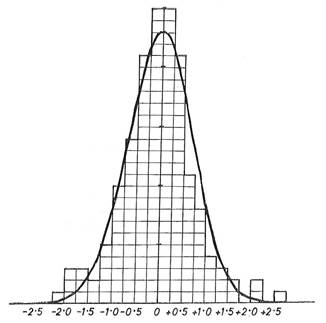
Figure 4. Adjustments to azimuths of 161 sections, in seconds.

Average adjustment 0".56. Normal distribution with distribution with

σ = 0.697 superimposed.

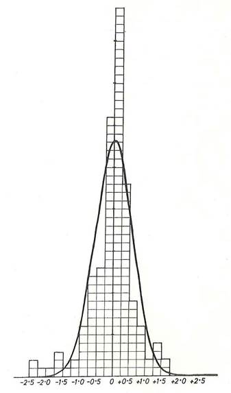
Figure 5. Adjustments to lengths of 161 sections, in metres.

Average adjustment 0.45 metres, or 1.4 parts per million.

Normal distribution with σ = 0.569 superimposed.

Analysis modified by common sense is a reasonable basis for decision in politics, management, and even engineering. Most surveyors, including the author, would prefer an analysis to which no modification was required. The methods here adopted were perhaps an advance on the Bowie method (Adams, 1930), where loops were adjusted separately in latitude and longitude, and no allowance for the varying standard errors of individual sections was made. The adjustments shown in Figures 4 and 5 give no major cause for dissatisfaction; yet the balance between forcing adjustments into distances on the one hand, or into azimuths on the other, was decided empirically, and on this subject the last word has not been said.

THE FORCED ADJUSTMENTS

Each section had now to be readjusted holding fixed the co-ordinates of its terminal junction points obtained from the National Adjustment. The aim was to produce one set of adjusted co-ordinates, and one only, for each of the 2506 stations, together with a unique set of adjusted angles, azimuths and distances. One or two precautions had to be taken. If there was a Laplace azimuth at a junction point whose longitude was amended by hand, then the Laplace azimuth had to be amended by hand also to maintain the Laplace condition. Moreover, the adjustment of a section holding single points fixed at each end is unsatisfactory.

TREATMENT OF JUNCTIONS

If the end of a section has to be adjusted laterally and only single points are held fixed at each end, a section without internal azimuths can simply rotate without distortion, and the whole of the adjustment is forced into the angles at the junctions - see Figure 6a, Moreover, more than one set of co-ordinates will be obtained for stations adjacent to the junction points. Accordingly, the azimuth and length of one line at each junction point was determined by taking the weighted mean of the azimuths and lengths obtained in the free adjustments. The co-ordinates of the far end of the line were computed, and the co-ordinates of both ends held fixed in all sections radiating from the junction - see Figure 6b (The longitude of each junction point having been changed by the National Adjustment, each of the azimuths obtained from the free adjustments had to be modified slightly to maintain the Laplace condition).

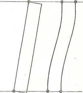
a b

Figure 6a & 6b. Distortion in forced adjustments.

As only one set of adjusted co-ordinates was to be obtained for any one point, any overlaps between sections included in the free adjustments were removed, except (in triangulation) for the junction point figure itself. For example, see Figure 7. The junction point is A, and the fixed line A-B. The south section can be adjusted immediately, holding A-B fixed. The west section can also be adjusted, holding A-B fixed, and including the quadrilateral A-B-C-D. In the forced adjustments of the north and east sections, the co-ordinates of C and. D would be held fixed as well as A and B.

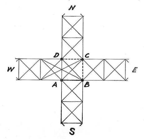
Figure 7. A junction of four sections of triangulation.

THE PUBLISHED ADJUSTMENTS

On the final runs of the forced adjustments, which were for general publication, diagnostic information of no interest to the general user was suppressed. All heights and distances were converted from feet to metres. Transverse Mercator co-ordinates and convergence were computed and listed on the output. Latitude and longitude were given to 0".0001, about 3 millimetres; azimuth and convergence to 0".01; easting, northing and distance to 1 millimetre; and height to 0.1 metre. It is not suggested that the observations justify so many decimal places; but it is permissible and convenient to define the geodetic model of Australia with high precision. For example, if the bearing and distance of a short line are computed from eastings and northings, satisfactory values are obtained.

The average adjustments to angles, azimuths and distances for four forced, adjustments in New South Wales and Victoria are shown in the bottom line of Table 1, where they can be compared with those obtained in the free adjustments. The average adjustments to directions and distances have increased very little, while the average adjustments to azimuths have been reduced. The constraints at the junction points seem to help the observed azimuths control swing in the intervening angles.

The last of the forced adjustments within Australia ran on 8 May 1966. The adjustment of New Guinea on the Australian Geodetic Datum immediately followed.

MISTAKES

Surveyors are paid to get the right answer and the wrong answer scores nought; yet the only man who can be quite certain of making no mistakes is the man who says nothing and does nothing. The data for the national adjustment is held on 20,000 cards, containing some 500,000 digits, and some mistakes have been made. The first adjustments of New Guinea had the Hiran distances in American feet instead of International feet, and had to be re-run. A dozen tellurometer lines in New South Wales had their chord-to-arc correction modified in one section, but correctly left alone in another. Mistakes in the tabulated heights and in the spelling of station names, which could not be subjected to mathematical check, are still occasionally detected.

Most of the larger adjustments shown in Figures 4 and 5, particularly those on the left side of Figure 5 which affect its symmetry, relate to sections where the field work is known to be of lower quality, and give no cause to suspect gross errors. But there are at least two places in Australia (loops 43 and 55), and three more in New Guinea, where the adjustments required are larger than can happily be attributed to the accumulation of random errors, yet despite intense searches no gross error has been found.

In addition to errors in the field work and in tabulating the data, it is possible for a mistake to lie hidden in a computer program, contaminating all work put through it. In some sciences, exact numerical tests of new programs are difficult or even impossible to devise, but surveyors are fortunate, and can arrange stringent tests. For example, one test of the variation of co-ordinates program was to check it against Rainsford's (1962) adjustment of the Ridgeway Base Extension, solution C. The adjustments agreed to 0".01 and 1mm. As Rainsford's adjustment was by condition equations, and the variation of co-ordinates program is by observation equations, this was a very convincing test.

With large programs which are frequently modified, it is tedious to retest the program comprehensively every time a small alteration is made; yet it is to inadequately tested modifications that mistakes, when eventually detected, have usually been traced. For several months, all adjustments reputedly run with a standard error for distances of 0.1feet plus 3 parts per million, were in fact run with a standard error of one unit. Using feet, the results were not so unreasonable as to attract attention, and the mistake was only found when an adjustment was repeated with distances in metres. Again, when the sign of grid convergence was arbitrarily changed, many subsequent adjustments had the sign of the convergence correct in the main part of the listing, but incorrect in the opening trig list.

ACCURACY

The methods and instruments used in the field suggest that the standard error between adjacent stations should be 3 or 4 parts per million, both linearly and laterally, and errors as great as 10 parts per million should be rare. As distances increase, the error expressed in parts per million tends to decrease, but not with the square root of the distance. The errors in a section are not all random. The error in azimuth tends to persist with the same sign at least from one Laplace station to the next. In. distance, the scale error due to our weak knowledge of geoidal height, and our ignorance of spheroidal height, will persist over large areas. Errors in crystal calibration, increasingly noted with the MRA2 tellurometer, may produce a scale error throughout a section. Dry temperatures measured at the terminals by day will never be too low; the ground is often hot to touch, and it is hard to believe that on average the recorded temperatures are not a little too high. An error of 1°F affects distances by about one part per million. However, the loop closures shown in Table 2 suggest that for distances of about 1000 miles, the average misclosure we can expect has reduced to about two parts per million, a foot for every 100 miles.

The variation of co-ordinates program does not compute the inverse matrix of the coefficients in the normal equations, so that it is not at present possible to quote the standard error of any one junction point with respect to any other. There seems to be little demand for information of this sort, but the theory now seems to be well understood, and if a demand develops, there should be no insuperable difficulty in writing the necessary program.

THE FUTURE

As additional observations are received in the years to come (notably, adjusted heights above the spheroid), it is foreseen that revised national adjustments will periodically be made. It is unlikely that every individual section will be readjusted in terms of each new national adjustment. Sections where there is scientific interest in highly accurate co-ordinates, such as those containing satellite tracking stations, can be readjusted; but it is not intended to issue revised coordinates for map control. Few things inconvenience cartographers more than frequent small changes in co-ordinates. The geodetic model of Australia obtained in 1966 seems free from plottable error at scales down to 1:25,000, and is likely to be retained for mapping and for a grid reference system for a long time.

MAINTENANCE OF MARKS

A geodetic survey is useless if the stations cannot be found on the ground. Clarke's triangulation of Great Britain had to be re-surveyed after less than a century, not because his work was inferior to that which replaced it, but simply because the majority of the marks were lost. Many of the geodetic survey stations in Australia are marked with solid stone cairns or concrete pillars, but many are not. In the rain forests of Queensland and among the sand ridges, marks have already been lost or destroyed. In New South Wales, permanent monument parties tour the geodetic survey, maintaining and improving the quality of the marks. Unless other survey authorities in Australia follow this example, much of the great work done in the last ten years will be wasted. The cost of maintenance, though not negligible, is far less than the cost of replacement.

THE FIELD WORK

Anyone who has rashly tried to compute an extensive triangulation scheme using the formulae of plane geometry will realise how easy it is for good observations to be ruined by inadequate theory. It is hoped that the present computations are worthy of the field work; but no theory, however involved, and no computer, however powerful, can obtain good loop closures from poor observations. Every reader of this paper will realise how much the geodetic survey of Australia owes to Dr. Wadley, the inventor of the tellurometer. The survey was planned and co-ordinated by the Director of National Mapping, in accordance with the recommendations of the National Mapping Council. It is the result of the efforts of many surveyors, both civil and military, from the Commonwealth and from the States, working sometimes in the mountains or by the sea, but often in the heat, the dust, the spinifex and the flies. In some parts of outback Australia, even 300 miles of tellurometer traverse can be a major journey, requiring great effort, and stressing everything, particularly vehicles, very highly - see Johnson (1964). When labouring in the office or at the computer, it has always pleased the author that some of his own field work is included in the adjustment, and that he played a part in this great enterprise.

ACKNOWLEDGMENTS

Anyone who undertakes the geodetic adjustment of a continent stands on the shoulders of his predecessors. The adjustment of Australia in 1966 evolved from the Bowie adjustment of the western U.S.A. in 1927 (Adams, 1930). The author had the benefit of a wonderful machine, the Control Data Corporation 3600 computer. In tackling the new problems brought about by the increased number of observed azimuths and distances, the author particularly acknowledges his great debt to his father, Brigadier G. Bomford, with whom he is in continual correspondence on many of the matters mentioned in this paper: Mr. B. P. Lambert made many good suggestions. Many people in the numerous survey authorities took great pains with the tabulation of the data. Finally, the author would like to acknowledge the part played by his computing staff of two surveyors, two technical officers, and two girls, who not only worked on the national adjustment, but computed National Mapping's own traverses and about 100 Laplace stations each year. Their work has been an admirable combination of high productivity and meticulous accuracy.

References

ACIC Technical Report No. 80, 1959: "Geodetic Distance and Azimuth Computations for Lines over 500 Miles"

Adams, O. S., 1930: "The Bowie Method of Triangulation Adjustment ". Special Publication No. 159, U.S. Coast and Geodetic Survey.

Allman, J. S. and Bennett, G. G., 1966: "Angles and Directions", Survey Review, No. 139.

Bomford, A. G., 1963a: "The Geodetic Adjustment of Australia: Progress to June 1963". Paper 23a presented to the Conference of Commonwealth Survey Officers, London. Reprinted in The Australian Surveyor, Vol. 20, No. 2, 1964.

----------------, 1963b: "The Woomera Geoid Surveys, 1962-63". Technical Report No. 3, Division of National Mapping, Canberra.

----------------, 1966a: "The Closure and Adjustments of the Geodetic Surveys in Australia". Ninth Australian Survey Congress, Perth, W.A. Duplicated.

----------------, 1966b: "Varycord: a Program for the Least Squares Adjustment of Surveys on the CDC 3600 Computer". Technical Report No. 6, Division of National Mapping, Canberra. In preparation.

Bomford, G., 1962: "Geodesy", 2nd Edition, Oxford University Press.

Fricke, W. and others, 1965: "Report to the Executive Committee of the Working Group on the System of Astronomical Constants". Bulletin Geodesique, No. 75.

Johnson, H. A., 1964: "Geodetic Survey through the Australian Sand Ridges", The Australian Surveyor, Vol. 20, No. 3.

Jordan, W. and Eggert, O., 1950: "Handbuch der Vermessungskund", Band II, Stuttgart. Lambert, B. P., 1962: "A Figure of the Earth for Australia", The Australian Surveyor, Vol. 19, No. 3.

Murphy, B. P., 1958: "The Least Squares Adjustment of Geodetic Figures with Observed Angles and Measured Sides", Empire Survey Review, No. 108.

Rainsford, H. F., 1957: "Survey Adjustments and Least Squares". Constable, London.

-----------------, 1962: "The Weighting of Telluormeter Lengths in Relation to Observed Angles", Empire Survey Review, No. 126.

Redfearn, J. C. B., 1948: "Transverse Mercator Formulae", Empire Survey Review, No. 69.

Robbins, A. R., 1962: "Long Lines on the Spheroid", Empire Survey Review, No. 125.

United States Air Force, 1965: "Special Report of Results, Australian Controlled Territory, South West Pacific Survey. Project AF 60-13". Three volumes. 1370th Photo-Mapping Wing, Air Photographic and Charting Service.

Veis, G., 1956: "The Deflections of the Vertical of Major Geodetic Datums and the Semi Major Axis of the Earth's Ellipsoid as Obtained from Satellite Observations", Bulletin Geodesique, No. 75, p. 140.