The Laser Years :
Recollecting Airborne Terrain Profiling for Photogrammetric Vertical Control
in the Division of National Mapping, 1962-1982
Compiled by Paul Wise, 2017-19
About this paper
This paper provides the most detailed account of the Division of National Mapping's airborne terrain profiling program that operated from 1962-1982. This program generated profiles of the terrain from which the location and height of selected points were extracted. These selected points were then used to control the aerial photography from which Natmap produced contoured 1: 100,000 scale topographic compilations.
While published papers about the profiling program are available they only reflected points in time whereas the story was a continuum. The continuum comes from the, possibly fallible, human recollection and this should be borne in mind by readers.
Acknowledgements
This paper was written with the valuable assistance of Natmapper and laser profiling party leader Rod Menzies. Input from Dave Abreu, Harry Baker, Ed Burke, Simon Cowling, Laurie Edebohls, John Ely, Oz Ertok, Andrew Hatfield, Graeme Lawrence, Michael Lloyd, Mike Morgan, Carl McMaster, Bill Stuchbery, Rom Vassil, and the support of Con Veenstra, John Manning, Syd Kirkby and Andrew Turk, is acknowleged. I am extremely grateful to Laurie McLean whose paper Recollections of the Aerodist Years provided a basic template and the impetus for this work.
About the author
Paul joined the Division of National Mapping as a Cadet Surveyor and remained with the Division and follow-on organisations for 30 years. He went on to become a senior and supervising surveyor, being involved with Nat Map’s terrain profiling operations, both radar and laser, for over ten years, and finally Director of Remote Sensing Operations at the Australian Centre for Remote Sensing (ACRES). Along the way he gained a Post Graduate Diploma (Aerial Photography) ITC Netherlands in 1983 and a Master of Engineering Science (Remote Sensing) UNSW 1988. In recent years, his work on the XNATMAP website saw him awarded a Medal of the Order of Australia (OAM) in 2016 for service to mapping and to mapping history.
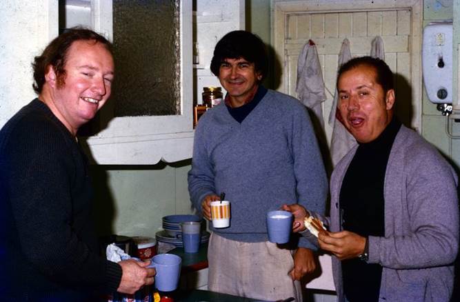
Long serving, laser terrain profiling personnel (L-R) Paul Wise, Rom Vassil and Ozcan Ertok during a break from flying operations at Esperance in 1974 (courtesy Laurie Edebohls).
|
Contents |
|
|
|
|
|
Chapter 2 - Evolution of Ground Based Vertical Control Acquisition |
|
Chapter 3 - Evolution of Airborne Vertical Control Acquisition |
|
|
|
Part 2 - National Mapping’s Use of Airborne Terrain Profiling for Vertical Control Acquisition |
|
Extracting Vertical Control from CARL Mark V, APR Terrain Profiles |
|
|
|
Chapter 5 – National Mapping’s Airborne Laser Terrain Profiling |
|
System Components comprising the Laser Terrain Profiler (LTP) |
|
|
|
Chapter 6 – National Mapping’s Second Generation Airborne Laser Terrain Profiler |
|
The End of National Mapping’s Airborne Terrain Profiling Operations |
|
|
|
|
|
|
|
Paper by Hocking, David Roy (1967), Photogrammetric Planimetric Adjustment |
|
Paper by Hocking, David Roy (1998), NATMAP Early Days, Map Compilation from Aerial Photographs 1948-1970s |
|
Operating Procedures for Analytical Aerial Triangulation |
|
Overview of Photographic Survey Corporation Limited of Canada |
|
Henry Correction : Its Derivation |
|
Laser Terrain Profiler : Technical Description |
|
Aircraft Modifications required to Grand Commander Aircraft prior to Fitment of Laser Terrain Profiler |
|
TIME CODE |
|
Nat Map’s Laser Terrain Profiling Yearly Progress |
|
Henry Correction Reimagined |
|
|
|
List of Figures |
|
|
Weapons Research Establishment designed decal rebranding their Laser Terrain Profiler, Mark 1, as WREMAPS1. |
|
|
Map index commonly known as the Red Line diagram. |
|
|
Diagram showing aerial photography acquisition with 60% forward overlap and 25% side overlap. |
|
|
Example of a photogrammetric or stereoscopic model. |
|
|
Map showing areas not covered by standard mapping photography after 1975. |
|
|
Diagrammatic representation of 7 photogrammetric models in an aerial photography flight strip. |
|
|
The Australian First Order Geodetic loops and lower order networks with mainland grid and offshore Aerodist stations for second order photogrammetric control. |
|
|
The Nat Map Aerodist lines measured. |
|
|
Map showing the Aerodist block adjustments and their identifier. |
|
|
Example of graphical radial triangulation or slotted template assembly. |
|
|
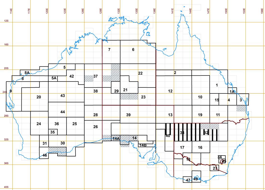
Photogrammetric Block boundaries and their numeric block identifier. |
|
|
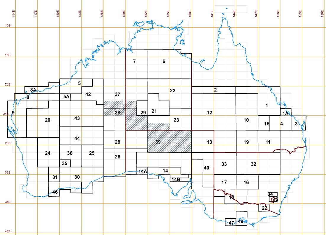
National Mapping’s Photogrammetric Blocks showing the blocks adjusted using the Slotted Template process and the blocks adjusted analytically. |
|
|
June 1971 photograph of the slotted template assembly for photogrammetric block 6 in the Rialto building in Melbourne. |
|
|
1979 photograph of National Mapping’s last slotted template assembly at Nat Map’s building in Dandenong. |
|
|
Indian Pattern Clinometer or the Tangent Clinometer. |
|
|
Showing the level planes at right angles to the plumb lines at two points on the earth's surface. |
|
|
Showing the relative heights of instruments and targets at two separate stations. |
|
|
Diagram showing an example of the optical mechanism automatically correcting the line of sight when the level’s telescope is tilted. |
|
|
A set of three aircraft altimeters being used for barometric heighting during astrofix operations and a precision Aneroid barometer. |
|
|
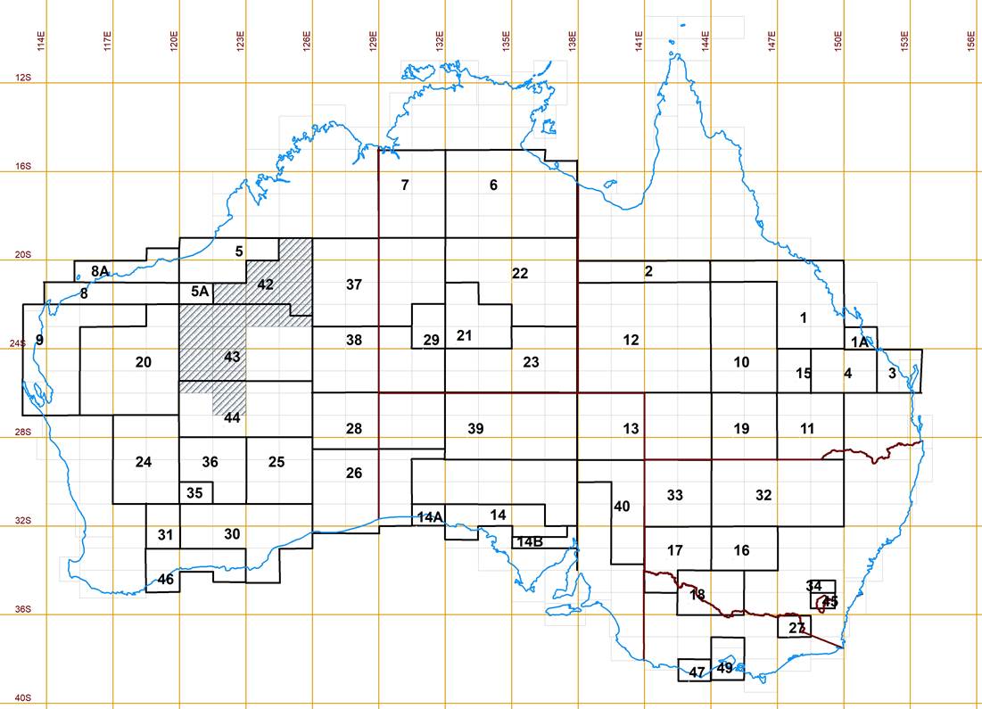
Photogrammetric Blocks which used barometric heighting techniques to provide vertical control for mapping. |
|
|
Sample of graphs for base and remote barometer readings. |
|
|
Schematic of components of WA-1M Automatic Altimeter. |
|
|
Nat Map’s Johnson Ground Elevation Meter. |
|
|
Trailer version of the Johnson Ground Elevation Meter. |
|
|
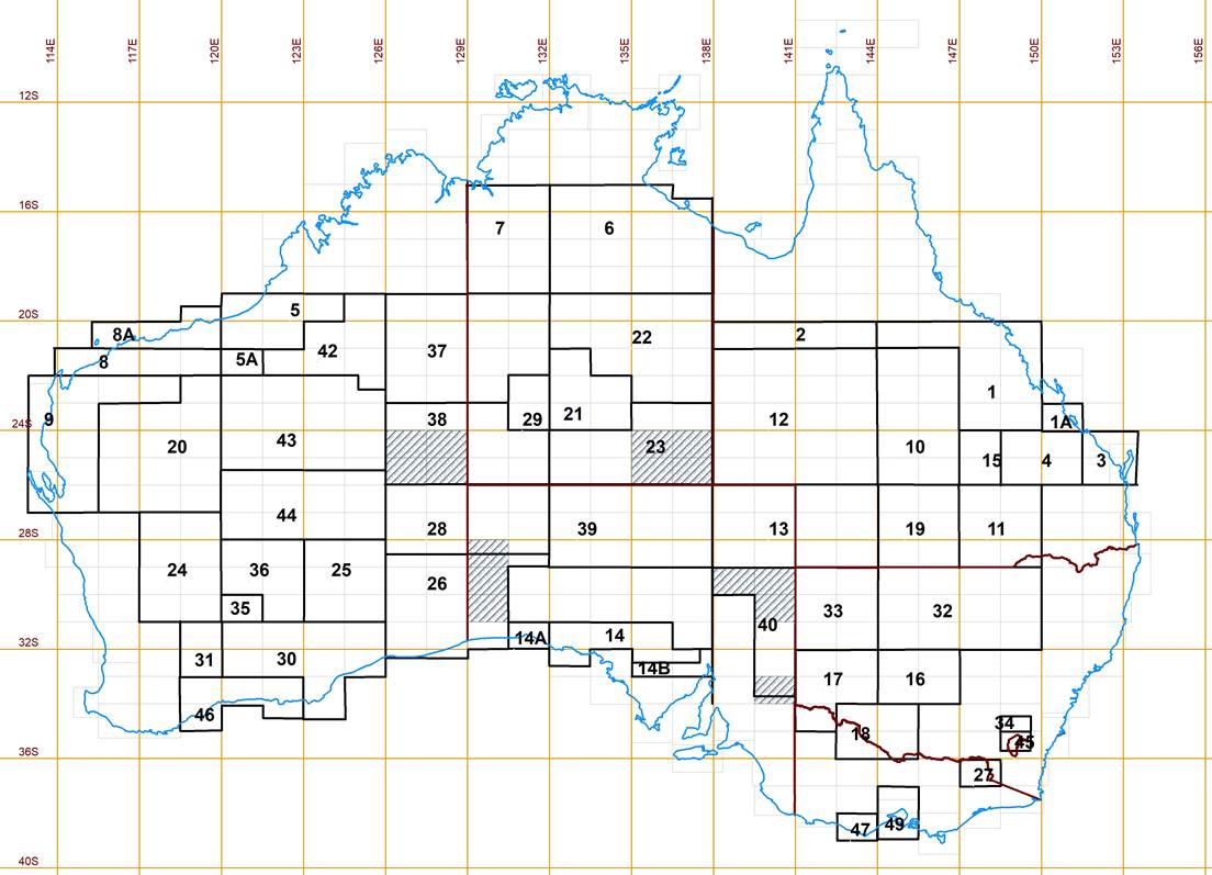
Photogrammetric Blocks which used heights obtained by Nat Map’s Johnson Ground Elevation Meter to provide vertical control for mapping. |
|
|
Configuration of an APN-1 Radio Altimeter. |
|
|
Canadian Applied Research Limited (CARL), Mark V, Airborne Profile Recorder instrumentation. |
|
|
APR operator’s console as mounted in the aircraft cabin. |
|
|
Example of an APR chart and associated 35mm film. |
|
|
Photograph of the APR operator’s console as mounted in the aircraft cabin of an ADASTRA Hudson. |
|
|
Diagrammatic view of the Henry Correction for the southern hemisphere. |
|
|
ADASTRA Lockheed Hudson VH-AGX. |
|
|
Example of APR flight line positioning in aerial photography sidelap. |
|
|
Example of the APR flight lines required for a standard 1: 250,000 scale map sheet of 8 strips of aerial photography. |
|
|
Map showing the 1: 250,000 scale map areas where contract APR was completed by ADASTRA for Nat Map. |
|
|
An artist’s impression of the laser profiler/receiver and electronics/services rack in an aircraft. |
|
|
One of the earliest Dakota trial laser profiles over Parafield airport near Adelaide. |
|
|
Contracted Executive Air Services, Rockwell 680FL Grand Commander VH-EXP, showing exterior signage over cabin door. |
|
|
Contracted Executive Air Services, Rockwell 680FL Grand Commander, VH-EXP on laser terrain profiling operations in 1975. |
|
|
Series of 1970 publicity photographs taken of the laser terrain profiler after installation in VH-EXP. |
|
|
Diagram showing respective operational configurations for VH-EXP and later VH-DNM. |
|
|
The profiler system installation in VH-DNM. |
|
|
The profiler assembly with laser tube, receiving telescope and slit camera. |
|
|
A laser tube with its transportation box. |
|
|
Section of 70mm Slit Camera photography. |
|
|
Operator’s panel on the profiler assembly. |
|
|
Electronic equipment and services rack with its modules. |
|
|
The timing code pulses and their translation into hours, minutes and seconds of elapsed time. |
|
|
Section of UV chart showing traces from the various instruments. |
|
|
Bendix B3 gyroscopically stabilised driftsight. |
|
|
Modified 4 ton Bedford RLCH 4x4 laser caravan from passenger’s side. |
|
|
Modified 4 ton Bedford RLCH 4x4 laser caravan from driver’s side. |
|
|
Laser caravan interior. |
|
|
International C1600 series four wheel drive with laser caravan. |
|
|
Ground power supply unit used to power the laser profiling system and the laser beam’s reflection in the lower photograph. |
|
|
Photograph at WRE. |
|
|
Laser profiling party ground transport Toyota Land Cruiser FJ55 series station wagon, ZSN003. |
|
|
Example of the LTP flight lines required for a standard 1: 250,000 scale map sheet of 8 strips of aerial photography. |
|
|
Third order levelling traverses of the Australian Height Datum (AHD) at 1971. |
|
|
Sample Survey Flight Record. |
|
|
Example of laser span calibration. |
|
|
Example of BRU calibration. |
|
|
Example of a Chart Breakout Sheet. |
|
|
Section of a laser profile chart. |
|
|
A sample calculation. |
|
|
Sample LTP Reduction form. |
|
|
Map showing the 1: 250,000 scale map areas where laser terrain profiling was completed between 1970 and 1975 in VH-EXP. |
|
|
Map showing the 1: 250,000 scale map areas where laser terrain profiling was completed between 1977 and 1979 in VH-DNM. |
|
|
Areas of Australia where terrain profiling by APR and LTP was acquired between 1962 and 1979. |
|
|
Thursday 9 September 1982 - the last laser chart. |
|
|
Map showing bases used by VH-EXP and VH-DNM for laser terrain profiling |
|
|
Natmap’s aerial survey platform Cessna 421, VH-DRB |
|
|
Photographs of the airborne and office components of the initial LAPS system. |
|
|
Map showing the 1: 250,000 scale map areas where PRAM/LAPS terrain profiling was completed in Cessna 421, VH-DRB. |
|
|
Graham and Ely with their Department of Administrative Services, Award for Excellence certificates |
|
|
|
|
|
List of Tables |
|
|
How the Henry correction is applied and misclose obtained for a profile line. |
|
|
|
|
Lasers have always been the stuff of science fiction and in the 1970s when National Mapping started using the Laser Terrain Profiler, the public still believed lasers were pure science fiction. The early Nat Map crews did nothing to dispel the laser myth with T-shirt logos depicting the world being cut in half by an airborne laser or saying that they could see from the air where they had previously profiled from the scorch marks their laser had left in the ground. It was only after the local cattlemen in a Northern Territory watering hole became so agitated by talk of a flying laser and threatened bodily harm to the profiling crew should any of their cattle be seen to be lost to this device, that crews became less boastful about the capabilities of this cutting edge equipment.
The term laser had originated as an acronym for light amplification by stimulated emission of radiation and the first laser had only appeared in 1960. Within ten years laser technology had been able to be adapted to practical uses including electronic distance measuring and cutting/welding. In Australia, the Weapons Research Establishment (WRE) of the then Department of Supply had their own programs researching laser adaptation.
National Mapping had already used laser based electronic distance measuring instruments to great effect measuring lines of around 50 kilometres in length to an accuracy of a few millimetres in a couple of hours. It was then no surprise to see that following a meeting between the Department of Supply and National Mapping in April 1966 that ground trials started in September 1967 on a laser terrain profiling system. Formal acceptance of the system by National Mapping occurred in July 1970. By around 1973 WRE had developed a more compact, modular airborne laser profiler for the Survey Corps of the Australian Army. WREMAPS as the laser terrain profiling system was officially named came from the same organisation who were world leaders in developing WREDAC, a digital computer, and WRESAT, an earth orbiting satellite.
Within some ten years the laser terrain profiler had completed its task for Nat Map. The lessons learnt by National Mapping in its struggle to adapt and maintain overseas equipment sourced from half a world away, saw the WRE locally made and maintained laser profiler an outstanding success. While much of the credit must rightfully go to Nat Map’s own electronics technicians who skilfully controlled the blue light, WRE’s Laser Group were unstinting in their efforts to minimise any disruption to the system’s flow of amps and volts. If the head count is right another sixty plus individuals contributed their own expertise at one time or another.
Working in the era when governments trained, employed and appreciated people expert in their fields and loyal to their vocation, the laser team quickly developed a culture that enabled them to be innovative, adaptive and to overcome any problem that could adversely affect their work. As an example, faced with a significant delay to operations when an engine of the Nomad aircraft had to be repaired following a 100 hourly service in Darwin, the field team didn’t hesitate to immediately assist the engineer to remove and crate up the offending engine. Then with the crate delicately balanced on the bonnet of a (privately hired) Mini Moke, and held in place by two people walking either side, they took it across the airfield and placed it in the hold of a passenger plane for transport to De Havilland in Sydney. Thus was saved considerable operational down time.
In the office accurate heights had to be extracted from sometimes wonky data and in the field, navigators worked hard to stay on course, technicians avoided blowing capacitors and camera operators ensured film cassettes didn’t jam. From such a concerted erffort the Laser program resulted in 250,000 kilometres of terrain profiles (approximately 6 times around the globe), a minimum of 100,000 height points being manually extracted and checked to permit the generation of 20 metre contours for the 1:100,000 scale mapping of the Australian mainland. Such an outcome stands as a testament to everyone involved and a job well done
This comprehensive and unique history, not only of the laser terrain profiler but also of the various technologies that predated it, is a credit to Paul.
Rod Menzies
February 2019
(National Mapping 1977-1987, Terrain Profiling Section 1977-1982)
Chapter 1 - Photogrammetric based Mapping for Australia
The majority of vertical control or points of known height, that the Commonwealth of Australia's Division of National Mapping required to produce contoured 1: 100,000 scale topographic national mapping, was obtained by airborne terrain profiling. Airborne terrain profiles were acquired over more than 70 per cent of the Australian mainland. Other methods were used to obtain vertical control over another 7 per cent of Australia, with the remaining area already having sufficient vertical control for generating contours at 1: 100,000 scale.
Airborne terrain profiling for vertical map control was, at the time, the most efficient method. More importantly it was necessitated by historical decisions made in the context of how Australia’s medium scale, national topographic mapping programs would be achieved. In his 1971 paper, Nat Map’s then Assistant Director Joe Lines posed the question why terrain profile recording? His answer was that the reasons lie fundamentally in the basic compilation technique originally adopted after an extensive testing programme some time ago. It was thus the decision to adopt the Arundel Method of map compilation that in turn led to the need for vertical control. At the time airborne terrain profiling was the only means of the timely and economical acquisition of such a volume of control for continental Australia.
Following World War 1 the British War Office had recognised the significance of aerial photography and the need to apply it to best advantage. In the late 1920s a captain in the Royal Engineers, and a brilliant mathematician Martin Hotine, later Brigadier Martin Hotine CMG CBE RE (1898–1968), was attached to the Air Survey Committee of the Geographical Section of the General Staff (GSGS) at the War Office. Hotine was one of a group of established mathematicians working on some of the problems associated with the simple graphical methods of surveying topographic information from vertical air photography. Thus was born the system of block photographic coverage by straight parallel strips, in some literature also called a run, in which each photograph in a strip overlapped its predecessor by at least 60%. Each subsequent parallel strip then also overlapped its predecessor by up to 25%. This forward and side overlap allowed the relief and aircraft distortions of a block of aerial photography to be rectified to established ground control by graphical means. The system of block, near vertical, aerial photographic acquisition and adjustment became known as the Arundel Method after the area in England where the idea was developed.
After receiving training from the Royal Air Force in 1926, Royal Australian Air Force (RAAF) Flight Lieutenant G Packer returned to Australia with these latest concepts in aerial photography acquisition and application. Packer subsequently became the RAAF’s chief adviser on aerial survey matters including the navigation and flying requirements fundamental to utilising the Arundel Method. Subsequently in 1931 the Australian Survey Corps produced the Albury 1 inch to 1 mile map sheet which was compiled with the significant aid of RAAF acquired aerial photography. When produced in 1936 however, it was the Sale 1 inch to 1 mile map sheet that was the first to be fully compiled from the Arundel Method of aerial photography acquisition and adjustment. Consequently, when the mid 1955 Recommended Plan of Mapping Operations was approved for a 1: 250,000 scale national topographic map series of Australia, the Arundel Method would be the basis for the series compilation.
The overwhelming problem that could not be solved for what became known as the R502 map series was how to supply all the vertical control that would be needed to enable the plotting of contours. At least one point of known height would have been required at a grid spacing of less than 10 kilometres or somewhere around 100,000 height points strategically located in relation to each aerial photograph. As there was no practical way at the time of acquiring these data, the R502 map series was produced with most map sheets devoid of contours and only having scattered spot heights. The second national Australian map coverage the National Topographic Map Series (NTMS) was to be contoured. As will be seen, by then enough work had been done to determine that airborne terrain profiling was the solution to obtaining the vertical control needed for the contour generation for the NTMS series.
Initially, vertical control for contouring the NTMS came from contract airborne profiles acquired using the Canadian Applied Research Limited (CARL) Mark V, Airborne Profile Recorder (APR). The APR system owned and operated by Adastra Airways of Sydney was contracted by Nat Map between 1962 and 1973 to acquire the necessary terrain profiles. Later, the Australian developed, Department of Supply, Weapons Research Establishment, Laser and Optics Section, Laser Terrain Profiler (LTP) Mark 1, was operated by National Mapping personnel from 1970 to 1979, to acquire airborne terrain profiles to complete the program of vertical control acquisition for the NTMS. The APR system used microwaves or radar as the basis of its height measuring system, whereas the LTP used a continuous wave laser. Thus, radar profiling as opposed to laser profiling can be found in the literature when referring to the use of APR and LTP. For clarity, WRE also developed a Mark 11, Laser Terrain Profiler for the Royal Australian Survey Corps. Soon after, Fairey Australasia Pty Ltd became the licensed manufacturer for future such equipment under the commercial name of WREMAPS. Nat Map’s laser profiler was then identified as WREMAPS1 and the Survey Corps’ as WREMAPS2. Nevertheless, for all its operational life Nat Map’s system was simply known as the laser terrain profiler (LTP) and that name will be used throughout this paper. Please refer to Figure 1 below.
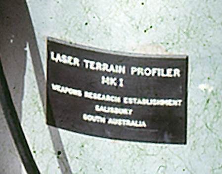
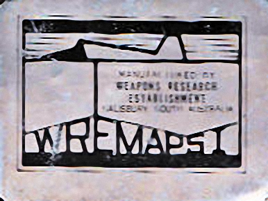
Figure 1 : Weapons Research Establishment designed decal rebranding their Laser Terrain Profiler, Mark 1, as WREMAPS1.
Like National Mapping’s Aerodist horizontal mapping control program, the airborne terrain profiling program was then thought to be a once only element in the national effort to have a topographic mapping coverage to meet Australia's then present and future requirements. Thus, Nat Map’s airborne terrain profiling program forms a major part of Australia's national mapping history. The first contract radar profile was flown in late 1962 in the Mount Coolon–Clermont area of Queensland and the last, in 1973 in South Australia - New South Wales. Nat Map flew its first laser profile in 1970 outside Broken Hill, New South Wales and its last south of Giles, Western Australia in 1979.
Airborne terrain profiling field parties usually comprised only a handful of people; a core group including pilot, to fly and operate the airborne equipment plus ground support when and where considered necessary. Apart from a suitable airstrip with aircraft fuel, only good flying conditions were required for airborne profiling operations. However, to extract the heights for photogrammetric model vertical control from both the contract radar and divisional laser terrain profiles an office component existed within Nat Map which also provided Nat Map field party support, planning and preparation, and contract management. Staff from this group were often rotated with the Nat Map laser airborne terrain profiling field staff.
Up to the end of 1976, Nat Map’s airborne terrain profiling operations were based at its Melbourne office in the Rialto Building at 497 Collins Street, Melbourne. From 1977 until 1982 when the last heights were extracted from the laser terrain profiles, airborne terrain profiling operations were based at its premises in Ellery House at 240 Thomas Street, Dandenong. As part of Nat Map’s 1977 change of office location, the radar terrain profiling material was sent to Commonwealth Archives as by this time all necessary height data had been extracted.
For the most part airborne terrain profiling operations were a function of the Topographic Surveys Branch of the Topographic Office. John Dunstan (Joe) Lines (Nat Map 1948-1976) was Assistant Director, Topographic Office to 1976, after which Sydney Lorrimar (Syd) Kirkby (Nat Map 1959-1984) took over the role. Orest Jacovlavich (Bob) Bobroff (Nat Map 1958-1982) initially headed the then Control Surveys Branch as supervising surveyor and later the Topographic Surveys Branch. From 1970, Rom Vassil (Nat Map 1965–1984) was the senior surveyor directly responsible for airborne terrain profiling operations. During 1967 and 1968 Rom had been engaged in vertical control field survey work with the Johnson Ground Elevation Meter. Rom replaced Edmond Francis Norman (Ted) Seton (Nat Map 1957-1970) on Ted’s decision to retire and return to his native Queensland.
Whilst having moved on in National Mapping by the time the Laser Terrain Profiler became operational the role of Leonard George (Len) Turner (1932-2002) should not be overlooked. As Supervising Surveyor (Topographic, 1966-1970), Len had carriage of horizontal control surveys and for vertical control surveys as well as other topographic mapping functions. Under Len, not only was the Aerodist system introduced (McLean, 2015), but contract airborne terrain profiling was evaluated and commenced. Further, Len instigated and managed Nat Map’s alliance with the Department of Supply’s, Weapons Research Establishment in developing the WREMAPS1 Laser Terrain Profiler. Two other Natmappers, Adrian John Wright (1944-2008) and Roderick William (Rod) Menzies (Nat Map 1976-1987) made significant contributions to Nat Map’s airborne laser terrain profiling operations; Adrian from 1971 to 1982 and Rod from 1976 to 1981. Electronics’ technicians John Ely (Nat Map 1966-1997), Ozcan Ertok (Nat Map 1971-1991), and Mick Skinner (Nat Map 1966-1973) were largely responsible for the operation and maintenance of Nat Map’s laser profiling system throughout its life. Their indepth knowledge of the various systems allowed minor failures to be rectified quickly and avoid significant downtime. The success of Nat Map’s airborne laser terrain profiling program is primarily due to their expertise.
After the 1977 internal reorganisation of the Melbourne based Topographic Office, Andrew Glen Turk (Nat Map 1969-1978) replaced Rom Vassil and with the later departure of both Bobroff and Turk, John Manning (Nat Map 1966-2004) as supervising surveyor and Paul Wise (Nat Map 1969-1987, airborne LTP 1972-1982) as senior surveyor oversaw the final years of the airborne laser terrain profiling program in National Mapping. A small lunchtime ceremony on 9 September 1982 marked the occasion of the completion of Nat Map’s airborne LTP program. Subsequently, with the move to digital mapping and stereodigitising data capture required to meet 1: 50,000 scale map accuracy standards, a second generation airborne terrain profiling system was then developed and this system is discussed later in this paper.
Photogrammetric based National Mapping
Photogrammetric mapping can be thought of as exploiting photographs, film or digital, as the primary data source for the provision of map detail. Although both aerial photographs and maps show an overview of the earth's surface, an aerial photograph is not a map (Crum, 1995). An aerial photograph is a perspective projection of the scene photographed. The position of detail in an aerial photograph is erroneous due to radial distortions caused by the optics of the camera, the relative instability of the aerial camera platform, and height differences in the terrain. For practical purposes, maps are directionally and geometrically accurate, given they show an orthogonal projection of a three dimensional world onto a two dimensional sheet of paper.
Through the principles of photogrammetry, the errors in near vertical aerial photography can be removed. The removal of these radial errors then permits the detail extracted from aerial photography to be accurately plotted, within the limits of the map scale, to make a map. Accurate extraction of the map information from aerial photography required that the aerial photography be controlled both horizontally and vertically. This horizontal and vertical control was provided by having points, in the terrain as well as identified in the aerial photography, with coordinates and/or height from purposely obtained survey data. For the most part, the acquisition of the aerial photography and its control was undertaken by separate programs dictated by the environment, technology and resources available at the time.
From time to time, various organisations including National Mapping, produced Orthophotomaps. Orthophotomaps were a mosaic of orthophotographs which were aerial photographs from which all the terrain, earth and camera related distortions had been removed and therefore all the features in the photograph were now truly positioned and to scale. For various reasons Orthophotomaps failed to meet the expectations of the producer and the user but can still be found in map libraries. The traditional paper line map has still to be replaced completely, despite technological advances.
After the Second World War, Australia embarked on its first national topographic map coverage at a scale of 1: 250,000. This coverage was known as the R502 series. While the R502 series derived its information entirely from aerial photography it was controlled horizontally by a mix of traditional survey, where available, and astronomic observations for position or astrofixes elsewhere. Only a few sheets were contoured (23%), as already mentioned, with spot heights derived from land and airborne barometric surveys shown on the remainder of the map sheets. Terrain was depicted by the method of hachuring or shading. The R502 mapping program had been underway for some ten years when in 1965 the Australian government decided to now accelerate the mapping program. Compilation of each map sheet (30 minutes of latitude by 30 minutes of longitude) would be at 1: 100,000 scale, with publication at both 1: 250,000 and 1: 100,000 scales. Importantly for many users both scales would now be contoured; at 20 metres vertical interval on the 1: 100,000 scale map sheets and 50 metres vertical interval on the 1: 250,000 scale maps. The production of contours for the whole of Australia within the planned timeframe however, would mean that traditional heighting techniques for providing the required vertical control would be inadequate.
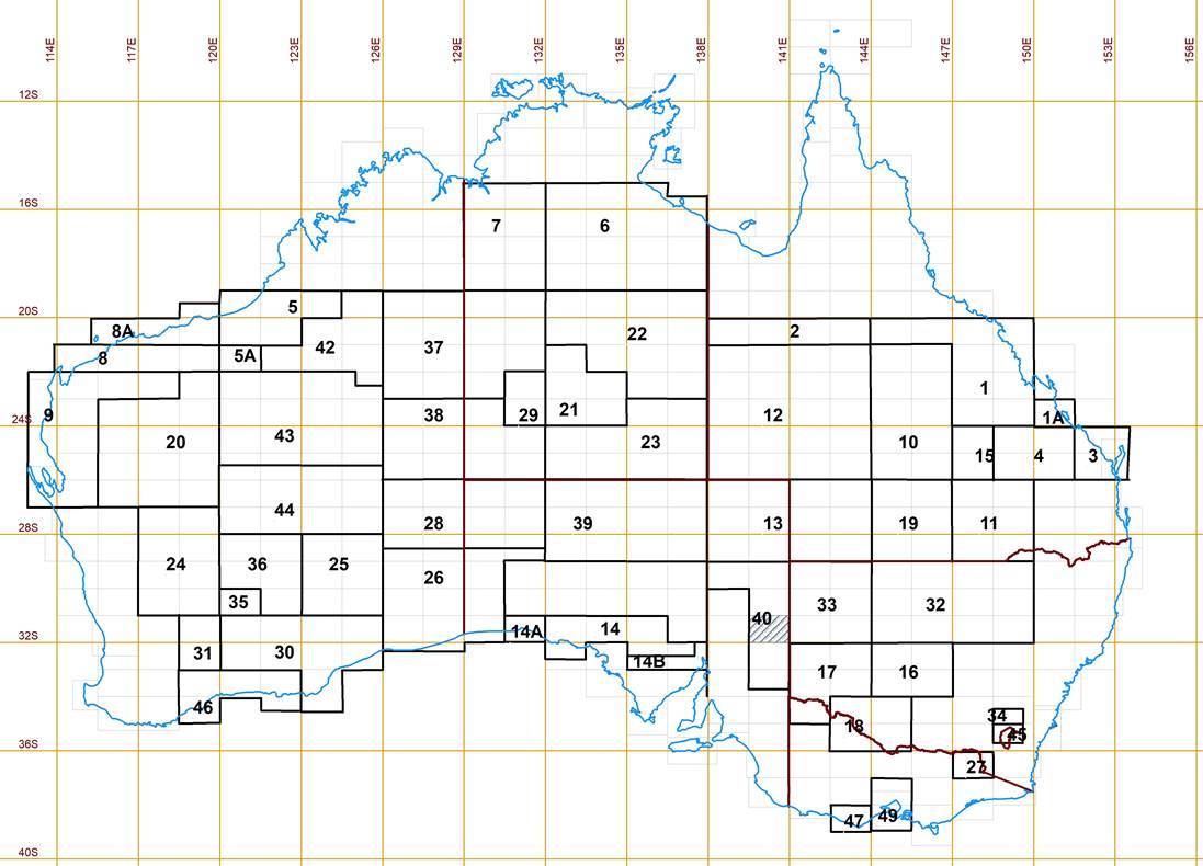
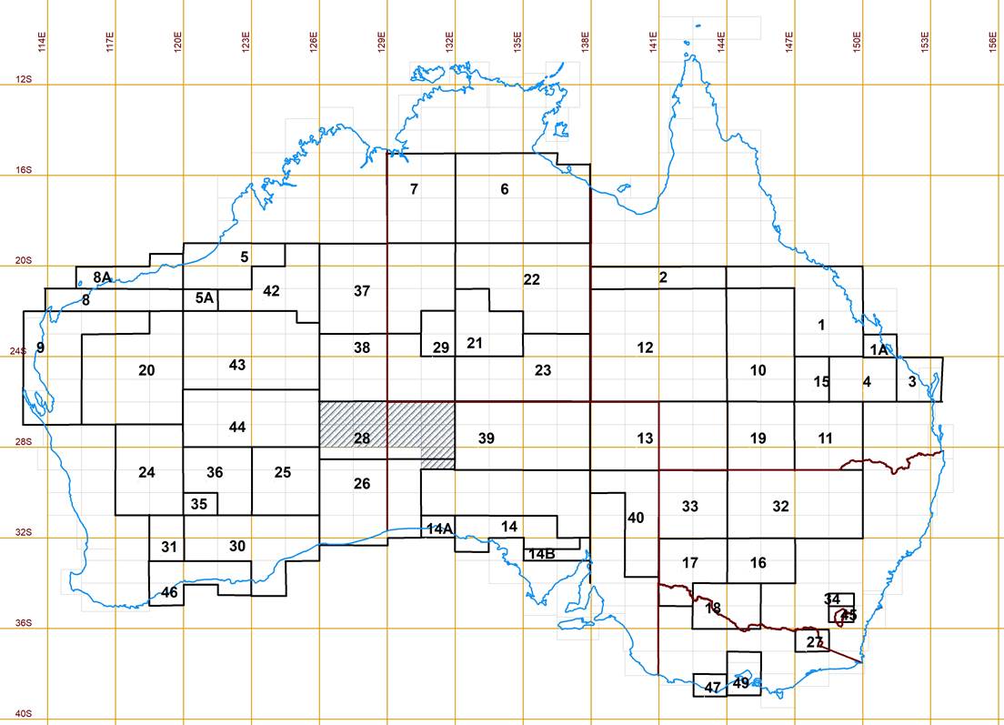
From the outset, resources allocated to this new mapping program, the National Topographic Map Series or NTMS, were never at the level required for the envisaged map publication schedule to be met. A more considered program was thus adopted being that all map sheets would still be compiled at 1: 100,000 scale but in the sparsely settled inland areas publication would only be at 1: 250,000 scale. Elsewhere, publication scale remained at 1: 100,000 scale. Figure 2 below shows a copy of the map with the thick red line the boundary between the two publication programs. (Only 1: 250,000 scale map publication would occur inside the red line on the diagram.) This map printed in red as shown in Figure 2, with its thick red line of demarcation became commonly known as the Red Line diagram. Notwithstanding the less than initially anticipated resource allocation, the NTMS program was hardly an inexpensive undertaking. The overall cost of the 1: 100,000 scale and 1: 250,000 scale maps produced under the program has been stated as A$600 million (O’Donnell, 2006).
The National Topographic Map Series at 1: 100,000 scale comprised some 3,062 map sheets which were completed around 1988. Some 1,460 map sheets covering the more remote inland of Australia were only produced to the compilation stage (O’Donnell, 2006). All 1: 100,000 scale compilations were used to derive new 1: 250,000 scale maps, gradually replacing the earlier R502 map series of the same scale. The 1: 250,000 scale NTMS program of 544 map sheets was completed in 1991.
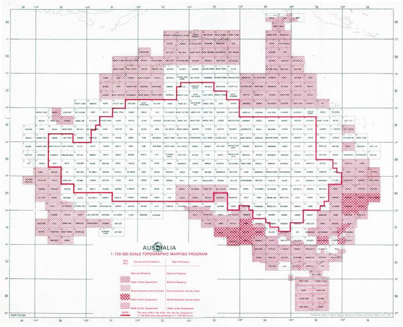
Figure 2 : Map index, commonly known as the Red Line diagram, showing the areas of responsibility for survey, compilation and map production as agreed by the National Mapping Council, in 1974.
This map further indicates that only 1: 250,000 scale publication would occur inside the thick red line on the diagram.
Aerial photography was again the primary data source for the NTMS program. The then technologically advanced Wild RC9 aerial survey camera replaced the K17 camera, or its equivalent. In the late 1950s, Wild Switzerland introduced the RC9 aerial survey camera with its superwide angle (nominally 88 millimetre focal length) lens and 230mm film format. When flown at 25,000 feet above sea level (ASL), the RC9 camera produced photographs with a nominal scale of 1: 80,000. The number of 1: 80,000 scale photogrammetric models covering a 1: 250,000 scale map area was approximately 70% less than the number of 1: 50,000 scale models from the K17 camera. (A photogrammetric or stereoscopic model generally consists of two aerial photographs that overlap by 60 per cent and provides a three dimensional view of the terrain). The reduced number of photogrammetric models to be controlled and used to plot the topography yielded flow on economies for other components of the NTMS program. Thus, the estimated overall cost effectiveness of 1: 80,000 scale photography was greater than that indicated by the reduction in the number of stereoscopic models alone (Lines, 1992). Given the magnitude of the NTMS program, such economies could not be ignored. Figure 3 below is a diagrammatic representation of aerial photography acquisition with 60% forward overlap and 25% side overlap. In Figure 4 below is an example of a photogrammetric or stereoscopic model consisting of two aerial photographs that overlap by 60 per cent. The coloured circles in the four corners show the areas where horizontal and vertical model control was optimally required.
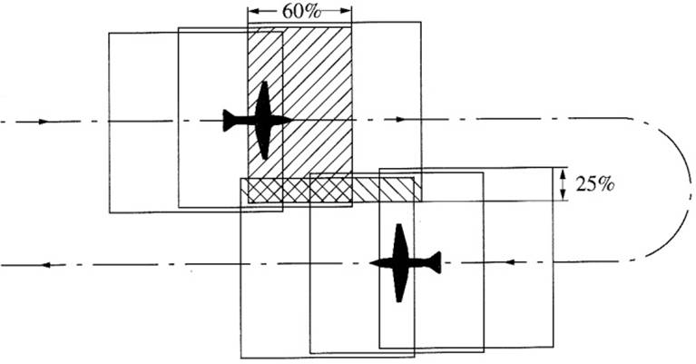
Figure 3 : Diagram showing aerial photography acquisition with 60% forward overlap and 25% side overlap.
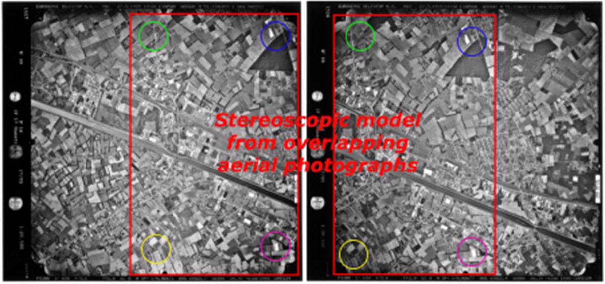
Figure 4 : Example of a photogrammetric or stereoscopic model consisting of two aerial photographs that overlap by 60 per cent.
The coloured circles in the four corners show the areas for optimal horizontal and vertical control.
A program thus commenced to acquire systematic, 1: 80,000 scale, monochrome, near vertical photographs of 1: 250,000 scale map sheet areas. Each such sheet area was covered by 8 or 9 parallel flight strips or runs from 25,000 feet (ASL) with the photography having a minimum of 80% forward overlap and 25% side overlap. As this aerial photography was to be acquired by private contractors, its provision was controlled by the National Mapping Council’s, Standard Specifications for Vertical Aerial Photography. Given the cost of logistics versus film and paper, the 80% forward overlap specification allowed a safety margin for meeting the minimum 60% forward overlap photogrammetric requirement. Between 1960 and 1975, all but the logistically difficult areas of Australia were captured on film as shown in Figure 5 below.
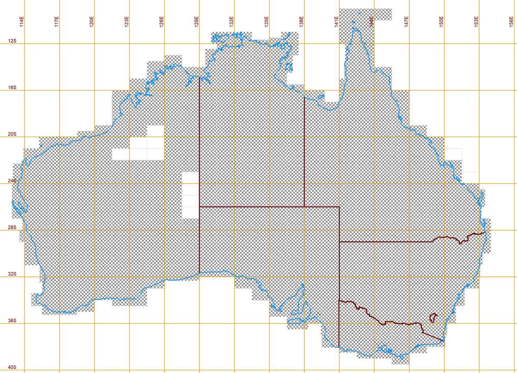
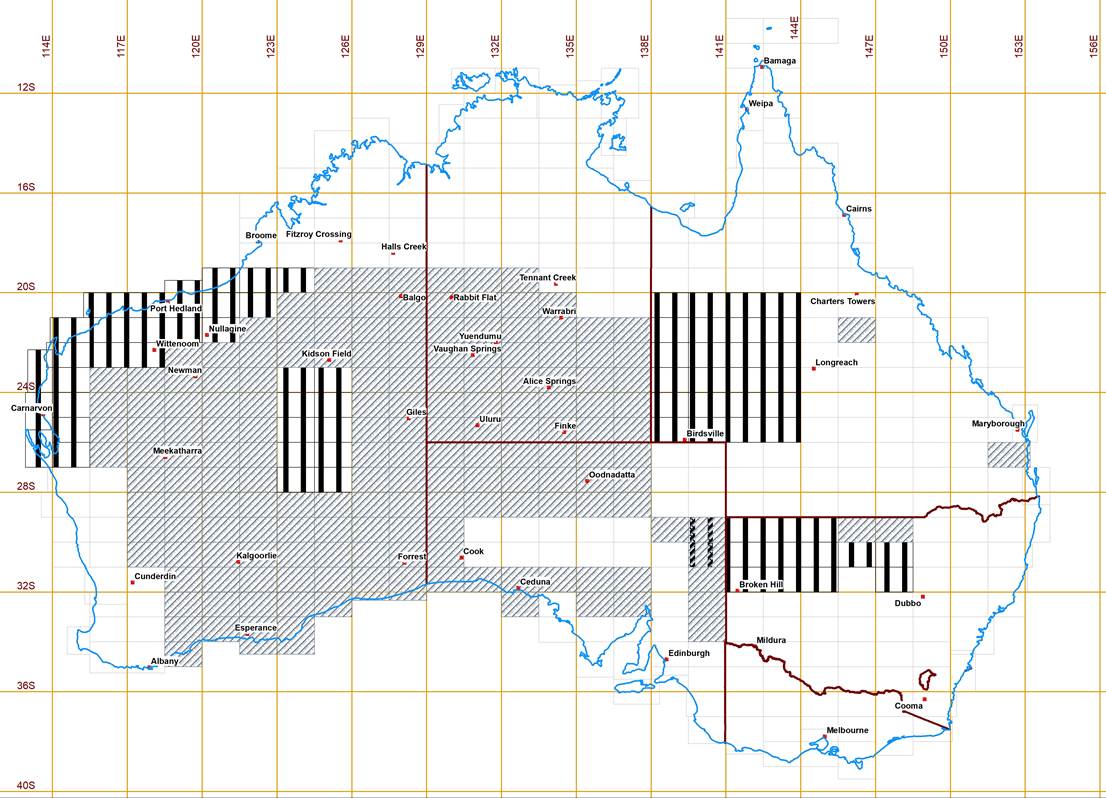
Figure 5 : Map showing areas not covered by standard mapping photography after 1975.
Although this aerial photography program reduced the number of photogrammetric models overall to be controlled and used to plot the topography and contours, each such photogrammetric model still required a minimum of four control points, located as indicated in Figure 4 above. These points, essentially three points plus one check point, with known position and height in the terrain would be sufficient to scale and orient each photogrammetric model. No technology then could effectively produce both position and height for the vast numbers of points in the terrain that would be required, so the processes for providing such control were separated. Horizontal and vertical control were acquired by separate programs and bought together at the photogrammetric plotting stage.
Figure 6 below is a diagrammatic representation of seven photogrammetric models in an aerial photography flight strip showing the indicative locations of both horizontal and vertical control points within the strip. As can be seen, separate to the control points are the respective photo centres, also called pass points, which appear on consecutive images within a single flight strip, and the pass, tie or wing points located near the model’s corners so as to be common to the applicable adjacent flight strip. The photo centre pass points along with the corner pass, tie or wing points enabled the individual photogrammetric models to be related to one another both along the flight strip and across flight strips. As can be seen more clearly in Figure 6, all the pass, tie or wing points are separate from the required horizontal and vertical (not shown) control points.
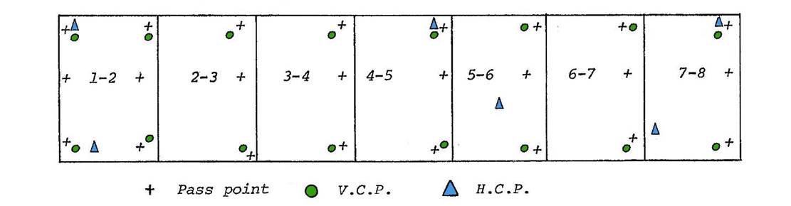
Figure 6 : Diagrammatic representation of 7 photogrammetric models in an aerial photography flight strip.
In the early 1960s, test work was carried out using a block of RC9 superwide angle aerial photography at a scale of about 1:40,000 in the vicinity of Canberra. This photogrammetric block lent itself to being controlled with varying densities of ground control, with superfluous control not used in each test to be used as an accuracy check on their positions as derived from each test. Extrapolating from this work, it was concluded that second order control spaced in the corners of geographic squares with sides of one degree of latitude and longitude would adequately provide the horizontal component for 1: 100,000 photogrammetric control. Each of these geographic squares would contain 4 x 1: 100,000 scale map sheets. Any additional control from the geodetic loops would be a bonus (Lines, 1992). Even so, on the vast, relatively flat regions of Australia establishing and surveying this required second order control was a daunting task. Aerodist or Airborne Distance measuring was the solution selected by National Mapping and became the technology behind the intensification of horizontal control for photogrammetric mapping.
Aerodist in National Mapping has been extensively covered by McLean (2015), so only a summary is provided here. In essence, the Aerodist airborne line measuring program and the intense sub program of Ground Marking for Aerodist resulted in a grid of Aerodist control points, or Aerodist stations, having coordinates to second order standard. Please refer to Figures 7 and 8 below. The horizontal adjustment of the Aerodist measured lines from each of the Aerodist stations to those Aerodist stations nearby and to the applicable existing first order geodetic control was done in blocks as shown in Figure 9 below. These Aerodist block adjustments (BA’s) were separate entities from the soon to be discussed photogrammetric blocks.
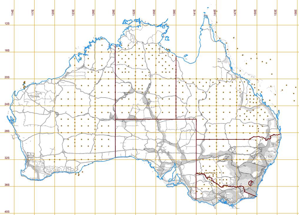
Figure 7 : The Australian First Order Geodetic loops (green triangles) and lower order networks (shaded grey) with mainland Aerodist station grid and offshore Aerodist stations for second order photogrammetric control.
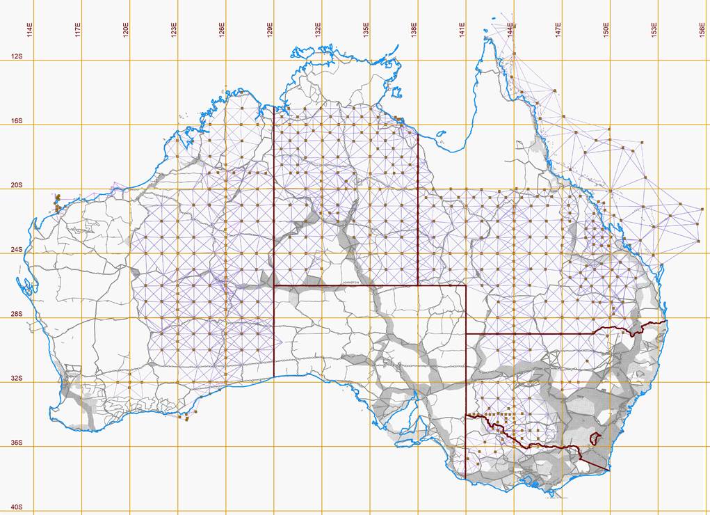
Figure 8 : The Nat Map Aerodist lines measured (purple lines) to enable the positions of the established Aerodist stations to be calculated.
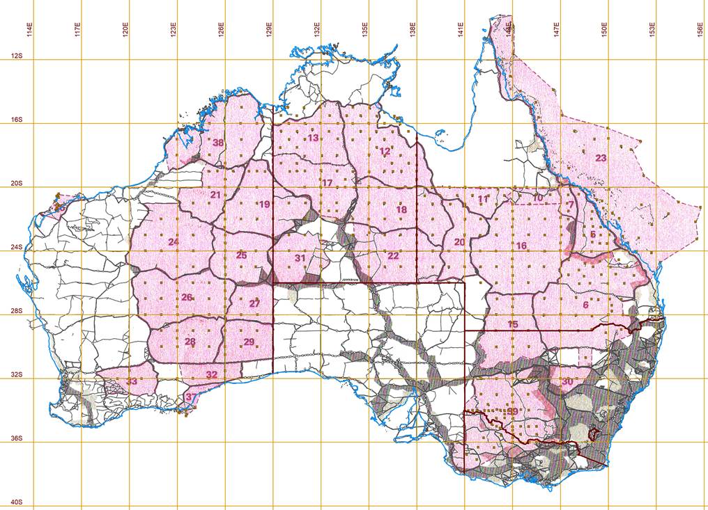
Figure 9 : Map showing the Aerodist block adjustments and their identifier.
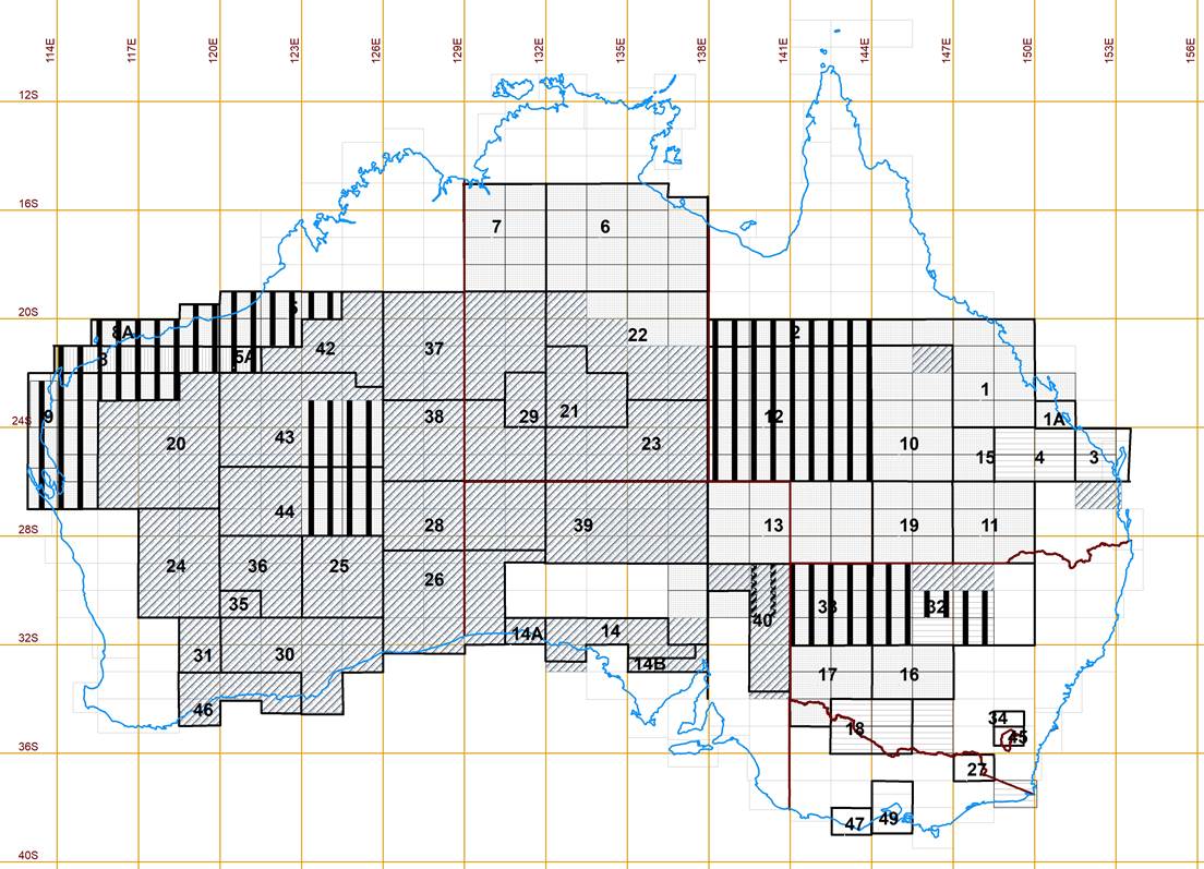
Demand, either real or perceived, was the driver behind the production and publication of the new NTMS. This explains why both Aerodist and airborne terrain profiling operations appear to randomly take place around Australia from year to year in no particular sequence. As explained above, the adoption of the Arundel Method by Nat Map meant that from its earliest years Nat Map had used graphical radial triangulation or commonly slotted templates to mechanically intensify the mainly perimeter horizontal control to the photogrammetric model level, within a photogrammetric block, as shown in Figure 10 below. Thus, a skill base had been developed within the organisation, allowing a mass production approach. Several assemblies or graphical photogrammetric block adjustments could be undertaken simultaneously using mainly radial templates which, with the inclusion of nadir templates, stereo templates and azimuth templates as necessary, met 1: 100,000 scale mapping accuracy requirements. Figure 12 : National Mapping’s Photogrammetric Blocks showing the blocks adjusted using the Slotted Template process (light hatches) and the blocks adjusted analytically (dark hatches). More detail about aerial photography acquisition, photogrammetric blocks, slotted template assemblies and stereoplotting may be found at Annexure A and Annexure B.
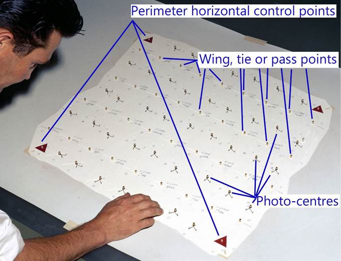
Figure 10 : Example of graphical radial triangulation or slotted template assembly.
The fixed perimeter control of the block is mechanically converted via the individual templates, to absolutely locate each photocenter and pass point at the final map scale.
A photogrammetric block comprised a number of adjacent 1: 250,000 scale map sheets. There was no specific size, rather the block’s extent was determined by the location of suitable horizontal perimeter control. Such control, Geodetic and/or Aerodist, had to be dense enough to prevent any outwards deformation of the block during adjustment. The photogrammetric blocks processed by National Mapping are shown in Figure 12 below. Later, when control intensification was undertaken using computer aided techniques the same use of perimeter control also enabled any large residuals to be highlighted during the analytical block adjustment. Figures 13 and 14 below show slotted template assemblies laid out.
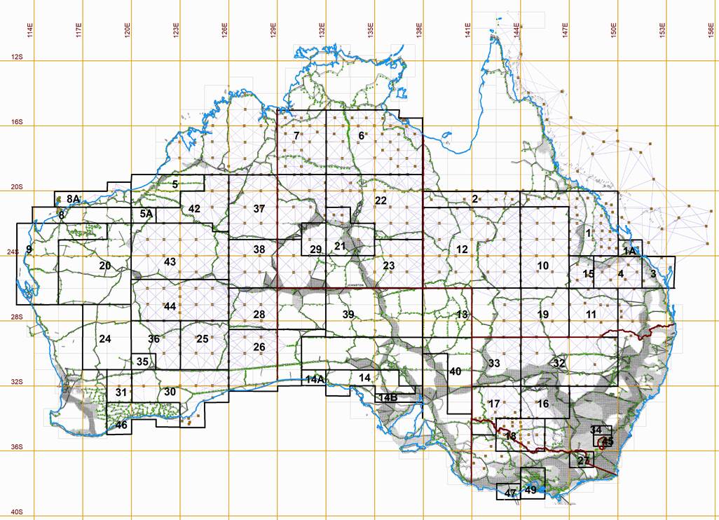
Figure 11 : The Australian First Order Geodetic (green triangles) and lower order networks (shaded grey) with the Nat Map Aerodist Horizontal Control network (brown points and purple lines) overlaid with the Photogrammetric Block boundaries and their numeric block identifier.
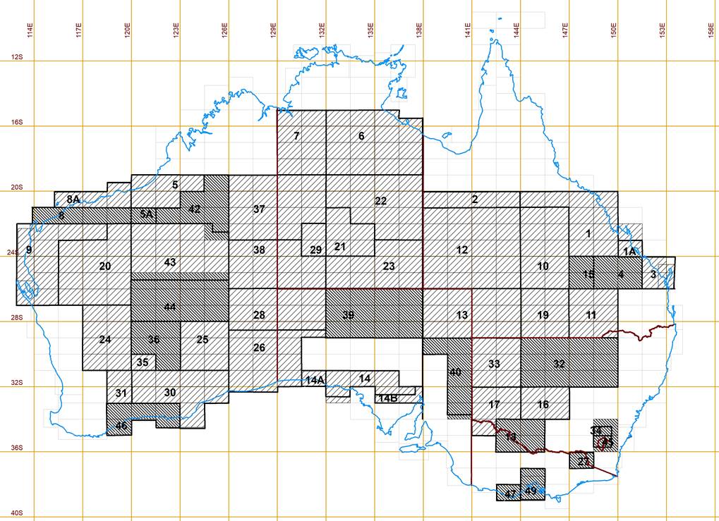
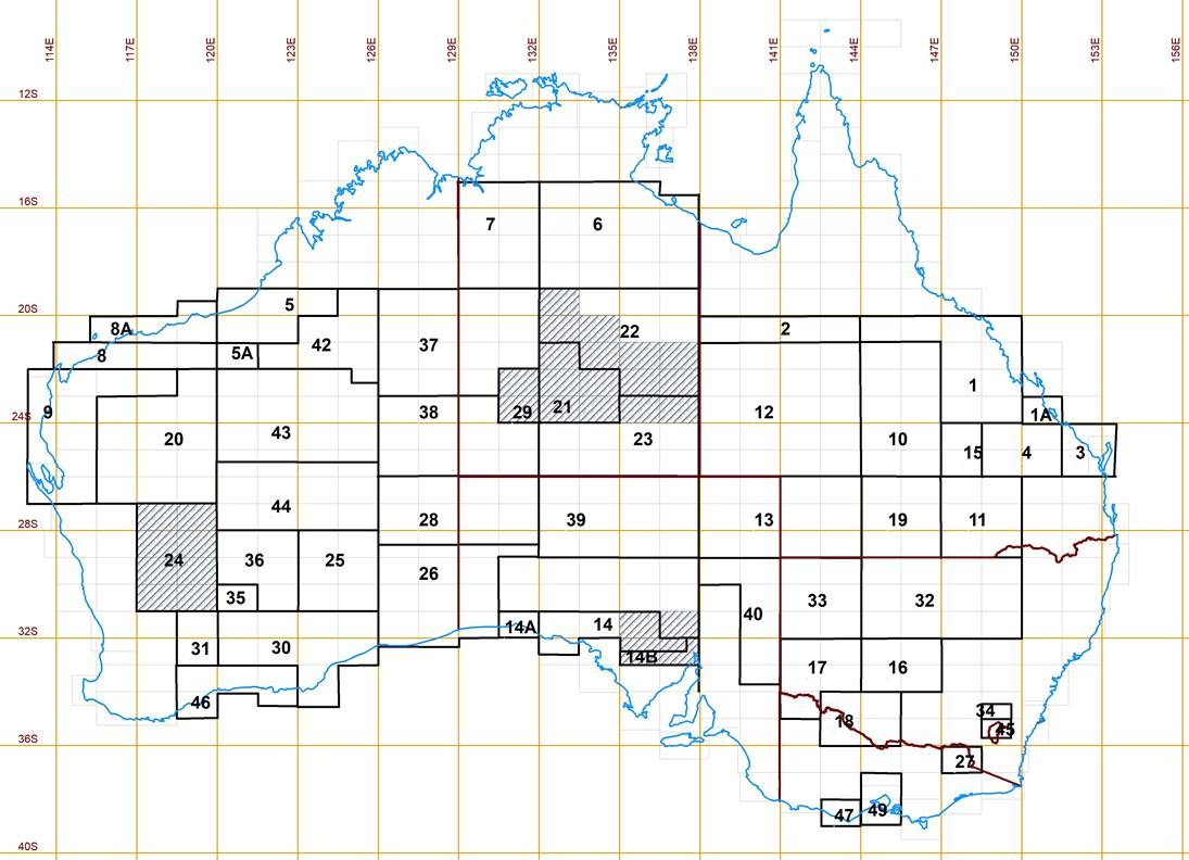
Figure 12 : National Mapping’s Photogrammetric Blocks showing the blocks adjusted using the Slotted Template process (light hatches) and the blocks adjusted analytically (dark hatches).
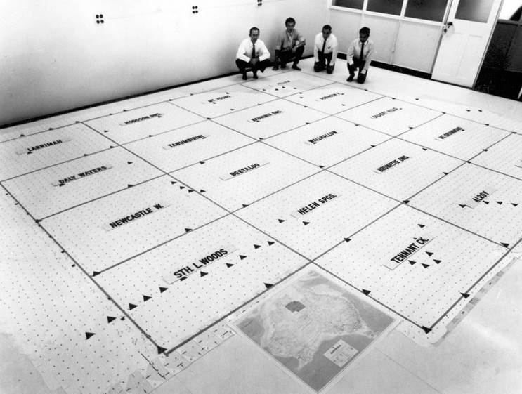
Figure 13 : June 1971 photograph of the slotted template assembly for photogrammetric block 6 with (L-R) Bob Foster, Ian Pasco, Len Bentley and Brian Martinesz, in the Rialto building in Melbourne.
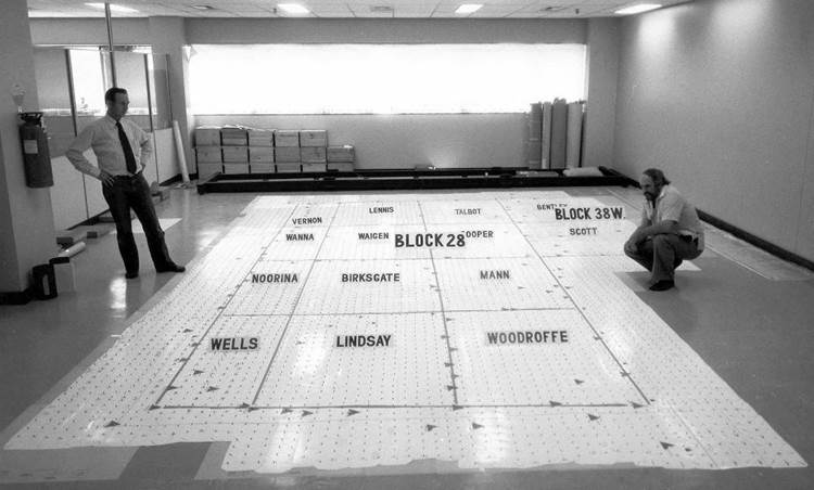
Figure 14 : 1979 photograph of National Mapping’s last slotted template assembly with (left) Bob Foster and (right) Dave Hocking at Nat Map’s building in Dandenong.
Vertical control was directly acquired in relation to the photogrammetric models comprising the block. With the aerial photography overlapping along and across each parallel flight strip, vertical control was optimised by having the heights of points in the four corners of the photogrammetric model as shown in Figure 4 above. A single height point could then be used as part of the control for up to four photogrammetric models (two along the flight strip and two on the adjacent flight strip). Vertical control for analytical block adjustments was acquired differently as is discussed below. Photogrammetric blocks thus became useful units for both contract and inhouse airborne terrain profiling operations, with the advantage that the data was collected at about the same time and with likely similar atmospheric conditions.
Analytical or Numerical Photogrammetric Adjustments
Some 52 photogrammetric block adjustments were undertaken by Nat Map. Analytical or numerical photogrammetric techniques were used to simultaneously intensify both the horizontal and vertical control in 17 of those blocks. Please refer to Figure 12 above.
National Mapping’s numerical photogrammetric MODel BLOCK (MODBLOCK) adjustment program along with FORMIT and MODSTRIP were developed by Dr CWB King from April 1972. Photogrammetric model joins within each strip of adjoining models were tested by the strip formation program FORMIT. Joins of strips of photogrammetric models to ground control, where applicable, were tested by the strip adjustment program MODSTRIP. The final join of strips to each other and to ground control was performed by the block adjustment program MODBLOCK.
King had originally developed MODBLOCK whilst Head of Photogrammetry and Mapping with the Iranian Oil Operating Companies in Teheran, Iran in the mid 1960s. MODBLOCK written in the FORTRAN computer language was able to compute a block adjustment of any size within the working space of eight method of least squares adjustment equations (King, 1967). The only additional storage requirement, over and above that of a single strip, was that for the solutions of each strip, but these were column vectors and not arrays. If there was any shortage of computer storage space, these data could be conveniently kept on a tape drive. At that time, King’s MODBLOCK ran on an IBM 7040, and utilised five tape drives for storage. While initially MODBLOCK ran on an IBM 1620, small storage, variable word length, decimal computer that was particularly suited to dealing with technical problems, MODBLOCK was subsequently expanded and improved to run on a UNIVAC 1108, and in Natmap ran on a Control Data Corporation (CDC) CYBER 76. With the introduction of mini and micro mainframe computers for Natmap’s digital mapping program, MODBLOCK was eventually able to be run inhouse.
While other numerical photogrammetric block adjustment programs existed their cost and adaptation were prohibitive to National Mapping. It was also considered that adjustment programs using the solution of polynomials were not sufficiently rigorous for Nat Map’s purposes. Such polynomial based programs assumed that the distortion in a strip was regular, which was not so. This disadvantage was of little import in a single strip where there was insufficient information to discover the true distortions. In a block adjustment, the many common points in the sidelaps of parallel strips gave a great deal of information as to the progress of distortion, which information was not fully utilised in a polynomial adjustment imposing regularity
The answer was a rigorous adjustment where all photogrammetric models, each with seven degrees of freedom, were adjusted simultaneously; or all photographs, each with six degrees of freedom, were adjusted simultaneously as in a bundle adjustment from comparator observations. This procedure involved the solution of many thousands of equations and would exceed the capacity of even large computers.
MODBLOCK was based on the seven unknowns of each independently observed model being solved simultaneously for all models of a block in a full least squares solution. The constraints were that all transformed values of observations of ground control points should as nearly as possible fit their true ground values, and that all transformed values of observed points in a model must as nearly as possible fit their transformed values in every adjacent model (if any) in which they also fall. This meant that each photogrammetric model was made to fit all its neighbours at once, irrespective of the way strips had been flown. This approach was clearly better than the polynomial method of forming up strips as a first step, without considering overlapping strips, and then holding the model connections fixed in the subsequent adjustment.
The number of equations to be formed and solved was still significant, but the process was broken down into stages that did not affect the rigour of the solution.
As the mapping photography to be used in the block adjustments was all flown east-west to cover a map sheet at 1: 250,000 scale and additionally had three north-south tie strips flown across each map area, the simultaneous adjustment of this pattern of photography permitted the amount of height control to be reduced. This fact impacted the operational acquisition of terrain profiling.
A feature that made the MODBLOCK program easy to use was that sorting routines had been incorporated. The user had only to select the two principal points and the two projection centres as the first four points of every model. Then any control, check or connection point between models of a strip, a tie point between strips or a single point was automatically discriminated. The final transformed coordinates were set out model by model for ease of plotting, with all common points correctly meaned over all the models in which they appeared. Within each model, points were sorted in order of ascending point name. Subsidiary programs plotted the vectors of residuals at control points and/or check points for visual interpretation of the validity of the adjustment and also plotted all transformed coordinates on base sheets for map compilation.
As mentioned above, the use of computer based adjustments meant that the laser profiling scheme could be reduced and was thus adjusted to a more evenly spaced grid. National Mapping’s approach was to establish horizontal and vertical control at the corners of units of about 120 models, which usually constituted areas about 100 square kilometres. Several of these units were enclosed within perimeter control for the block. Perimeter control was usually the 1° or 30¢ network of trig points with vertical control provided at a spacing of 4 to 6 models (about 60 kilometres) along all flight strips.
In areas which were to be adjusted by numerical photogrammetric techniques the terrain profiling pattern was therefore planned so as to acquire profiles along the block perimeter and then approximately equidistant, not exceeding 60 kilometre intervals, between those limits. This resulted in an almost square grid of profiles over the block. As there was more flexibility in where the profiles could be obtained, where possible all profiles were planned to overfly as much existing vertical ground control as possible. More detail may be found at Annexure C.
For the most part however, Nat Map’s airborne laser terrain profiling operations were undertaken as described in Part 2 below.
Chapter 2 - Evolution of Ground Based Vertical Control Acquisition
Vertical Control from Optical Observations
The difference in height between two points was traditionally found by angle and distance measurement from the first point to the second point and simple trigonometry. The Indian Pattern Clinometer or the Tangent Clinometer as shown in Figure 15, measured the angle of elevation or depression and also gave its tangent. As the height difference between the point of observation and that being observed was distance to the observed point by the tangent of the angle read by the clinometer, having the tangent easily readable as well as the angle meant no tables needed be carried. The two vanes folded down for portability.
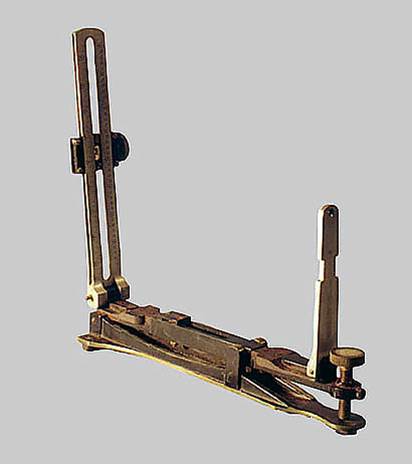
Figure 15 : Indian Pattern Clinometer or the Tangent Clinometer showing the eye vane right and object vane left, engraved with the angle and its tangent.
This method developed into a technique called Simultaneous Reciprocal Vertical Angles. The technique relied on the vertical angles being read simultaneously at each point to the other thus removing any atmospheric effects. This technique was largely used on geodetic surveys to carry height from point to point using theodolites to accurately obtain the angles at both end points to the other.
Nat Map specified that Simultaneous Reciprocal Vertical Angles be observed when the air was most evenly heated. This was not before about 2 hours after the sun had crossed the meridian in the area, and not later than about 4 to 4½ hours after the sun had crossed the meridian. In practice, between 2 and 3PM was a good time in the days observing routine. As shown in Figure 16 below, the vertical angles observed during a geodetic survey were nearly always angles of depression.
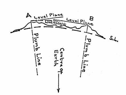
Figure 16 : Showing the level planes at right angles to the plumb lines at two points on the earth's surface.
Note that the line of sight is below this plane at both points and thus the vertical angles observed were nearly always angles of depression.
For field computations the following formula was adopted to compute the height difference between stations. It was based on two assumptions; one, that for the small vertical angles normally involved, the mathematical Sine and Tan functions of the angles are the same, and two, the slope distance and horizontal distance between the two points were almost the same, so no inaccuracy is introduced by using the Tan function and the slope distance between stations as measured by electronic instruments. The formula was, for two stations A and B and taking the signs of the observed vertical angles into account :
Difference in Height = Slope Distance A-B x Tan½ (Angle at A - Angle at B)
If there was a considerable difference in height between the two stations the problem was resolved by initially using the above formula to calculate the approximate height of the forward station B. Using the now known heights of both stations to convert the slope distance to the horizontal distance, and then recomputing the heights with this accurate horizontal distance and the Sine function instead of the Tan function of the vertical angles. It was important that distances were not reduced to sea level for these height computations.
In determining heights from Simultaneous Reciprocal Vertical Angles one final correction was required. This correction was required because the angles were observed by two separate instruments to two different targets all set at different heights in relation to the height of the respective station marks as shown in Figure 17 below.
Instrument and Target Correction = (Instrument height at A - Instrument height at B + Target height at A - Target height at B) / 2
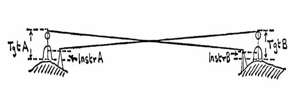
Figure 17 : Showing the relative heights of instruments and targets at two separate stations.
As instrumentation developed, spirit levels evolved where a bubble was used to indicate a horizontal plane about a point. By reading where this plane intersected a graduated staff held vertically over another point, the height difference between the two points could be determined. The evolution of this technique was called spirit levelling or just levelling. The introduction of automatic levels greatly improved the speed and accuracy of a levelling survey. The use of automatic levels reduced the time taken and human inaccuracy in the centring of the level’s bubble i.e. setting the horizontal plane. The automatic level had a prism which swung freely and thus under the force of gravity set the horizontal plane. A damper was incorporated to steady the line of sight and the whole unit of prism and damper was called the optical stabiliser. Once the instrument was set approximately horizontal using its small circular (pill) bubble, the optical stabiliser could then itself swing automatically into a position that set the true horizontal line of sight. A diagram showing this optical/mechanical solution is at Figure 18 below. Even with this development acquiring the vertical control needed for photogrammetric mapping was far too slow. Nevertheless, like the loops of the geodetic survey which provided a national set of fixed, homogenous positions on a single national datum, loops of third order levelling provided a similar set of fixed, homogenous height points on the Australian Height Datum (AHD). Again, like their horizontal counterpart, these loops of heights were too sparse to be used as photogrammetric control but were the basis for controlling the vertical control or height intensification programs as will be discussed.
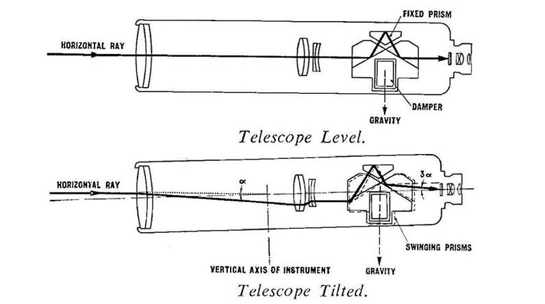
Figure 18 : Diagram showing an example of the optical mechanism automatically correcting the line of sight when the level’s telescope is tilted.
Rather than the instrument man and staff men walking between their respective observing and setup locations motorised vehicles were sometimes used. The most sophisticated version used specially modified vehicles to mount and transport the levelling equipment and operators. These vehicles allowed for the rapid setup and observation without leaving the vehicles. In 1983 the United States reported on their testing of this equipment in their paper A Test of the Swedish Motorized Levelling System presented at the 10th United Nations Regional Cartographic Conference Asia and the Far East.
Vertical Control from Barometric Heighting
Barometers had been seen as an alternative to levelling. Provided the atmospherics were favourable, barometers could be carried from point to point very easily and from their readings height differences obtained. After World War Two, surplus aircraft altimeters increased the availability of pressure sensitive instruments and the aircraft altimeter had the advantage of having an increased vertical range as compared to the barometer. The word barometer will be used hereonin to refer to both types of instrument. Three barometers were usually mounted in a box for ease of transportation and so as to be able to identify a failure in any instrument. With one set of three barometers at a base station, usually of already known height, a roving set or sets of barometers would be transported to points where heights were required, as shown in Figure 19 below. Later comparison of the readings would allow heights of the points visited to be calculated.
Barometric heighting was used during the astrofix acquisition program for the R502 mapping program. Barometric observations were taken by astrofix parties at creek crossings, homesteads and airstrips to provide some indication of the extent of the relief in an area. With the availability of light aircraft and helicopters the barometric heighting technique evolved further.
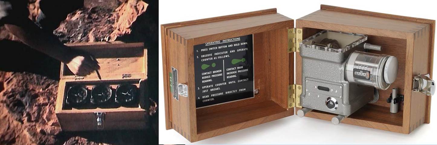
Figure 19 : (Left courtesy Peter Hocking) A set of three aircraft altimeters being used for barometric heighting during astrofix operations.
(Right) A precision Aneroid barometer by Mechanism Limited of Croydon, UK, as used by Nat Map in the 1960s and 1970s.
In the 1950s, the Department of the Interior was requested to assist the Bureau of Mineral Resources (BMR) with survey control for the network of gravity measurements being planned across Australia. For gravity purposes, BMR were to establish, by helicopter borne barometric observation, stations on an approximate 7 mile by 7 mile grid. As height at each such station was necessary for the reduction of the gravity data, the grids of spot heights that emerged from this work became of value to topographic mapping and charting. Several hundred thousand square kilometres of sedimentary basins in Western Australia, Northern Territory and western Queensland were covered in this manner by helicopter borne survey parties (Lines, 1992).
In the reduction of the gravity observations, heights with errors in excess of 1 metre above mean sea level became significant. Height control was therefore provided by levelling traverses along roads and tracks in the area of the survey. This levelling was carried out by the Department of the Interior. Not only did this work assist the gravity surveys but also contributed to loops of levelling used for later establishing the Australian Height Datum.
The only photogrammetric blocks recorded as being controlled by barometric heighting in National Mapping, were Blocks 5A and 8 as shown in Figure 17 below. This work was done in 1968 by a field party led by Ted Seton which used a helicopter to obtain observations at the required points. For this work, and all future work needing accurate atmospheric pressure readings, Nat Map used the Aneroid barometer by Mechanism Limited of Croydon, UK, as shown in Figure 16 above.
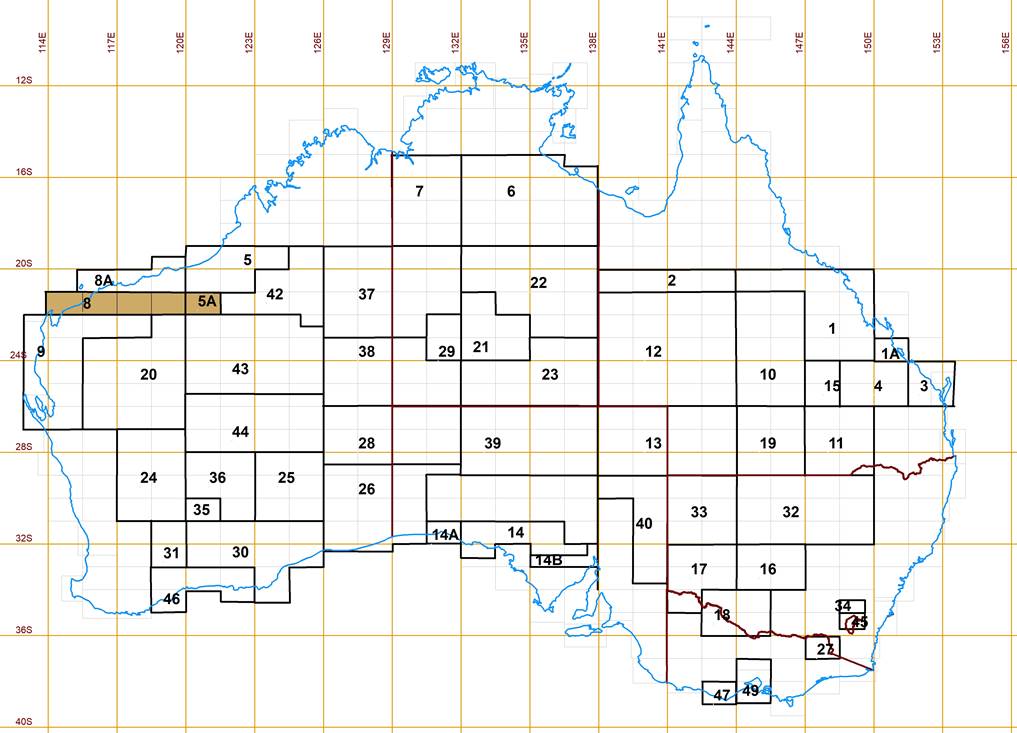
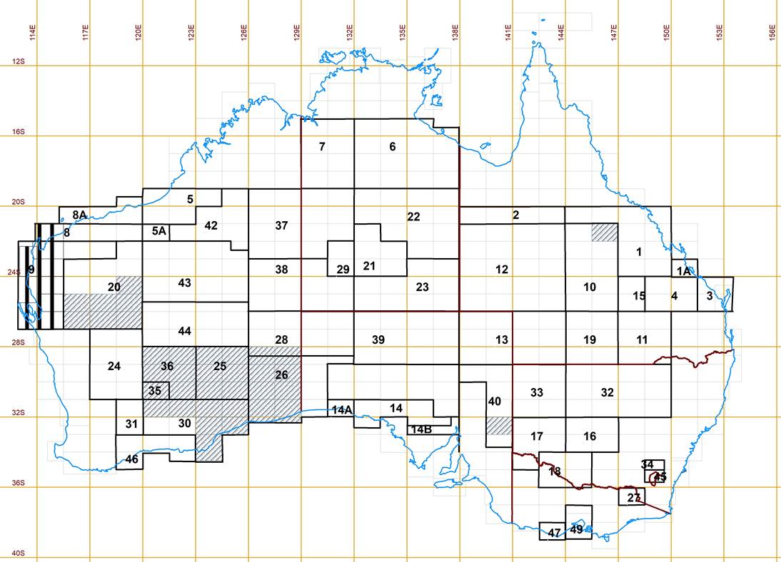
Figure 20 : Photogrammetric Blocks which used barometric heighting techniques to provide vertical control for mapping.
The so called Mechanism Barometer had a digital readout of the pressure direct to 0.1 millibar. Reading errors were thus largely eliminated, but to avoid instrument failure or mishandling, readings from two instruments were taken at all points during a barometric survey. With these instruments, National Mapping’s approach was generally to read all base and roving barometers at the base station before departure, read all barometers at hourly intervals while the roving barometers were at their distant location(s), and then read all base and remote barometers on return of the roving barometers to the base station. The base station was generally located near to a bench mark or other point of already known height. If hourly readings were not possible at the remote location(s) then a graph of the readings at the base station was drawn to permit interpolated base station readings to be obtained for the same instant of time as the remote readings. It was normal practise to draw a graph of both base and remote station readings, as shown in Figure 21 below. If then the graphed curves were not generally parallel, unsuitable weather conditions, or errors in reading the barometers were indicated and unreliable heights could be expected. Each time the atmospheric pressure was observed ambient air temperature was also recorded.
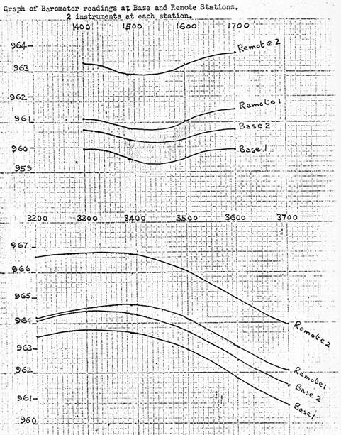
Figure 21 : Sample of graphs for base and remote barometer readings.
Computation of final heights used formulae documented by Lt Col CA Biddle, RE, Senior Lecturer in Surveying, University College, London (Biddle, circa 1960s). Simplistically :
(height at point b – height at point a) = KTv (log(pa/pb))
where pa and pb were the pressures (millibars), at each station respectively.
At the time logarithmic (log) tables were widely used and since such tables were required for one term in the above formula, it was very convenient to complete the computation by logs. Hence :
log (hb – ha) = log (KTv) + log (log pa – log pb)
To simplify the calculation further a table of log (KTv) values was prepared for a range of values of temperature in degrees Celsius where :
log KTv = log (221.266 *(°C + 273)) for heights in feet, or
log KTv = log (67.442 *(°C + 273)) for heights in metres.
When calculating machines became more readily available, the formulae used were :
Difference in height (feet) = Difference in pressure x (Temp °C +273) x 221.266, or
Difference in height (metres) = Difference in pressure x (Temp °C +273) x 67.442.
Again to simplify the calculation further tables of (Temp °C +273) x 221.266 and (Temp °C +273) x 67.442 for a range of values of temperature in degrees Celsius, where prepared.
Toward the end of the 1950s aerial photography and photogrammetric techniques were commanding an increase in accuracy, specifically that of vertical control. Technological evolution in engineering, electronics, and materials saw the implementation of new ground and airborne data gathering.
Vertical Control by Specialised Vehicle
Deumlich (1982), outlined the then Soviet WA-1 or Automatic Altimeter, which not only computed the elevation differences when driving over the terrain but also recorded the profile of the path covered and permitted the reading of elevations and elevation differences on counters. Please refer to Figure 22 below. This circa late 1950s device used a pendulum for outputting impulses proportional to the slope angle and using a measuring wheel to determine distance travelled. The profile was recorded on a roll of photographic paper. Up to 90 kilometres could be profiled in a seven hour day and with the later WA-56 instrument an accuracy of ±4 to ±10 centimetres could be achieved with double running and slopes between ±15 degrees.
Figure 19 shows the pendulum (1) which ended in a thin wire touching a globoidal drum (2) uniformly rotated by a motor (3). The groove (4) represented a contact line. A relay (5) was operated by every contact with the pendulum wire. The distance measurement was made by determining the revolutions of the wheel (9). The result was also conducted by the reductor (8) to the integration sockets (6) and (7), their rotation being controlled by the redactor; (10) represented the armature of the socket. Elevation was measured by counter (11), the travelled road distance by counter (12). The result of the levelling was recorded on a tape of photographic paper (15). The optical system of projection was indicated in (14). The light cylinder (13) effected the transformation of the angle of rotation into a linear displacement. It consisted of an opaque cylinder, the surface of which was pierced by screw-lines at two diametrically opposite places. As a result, an automatically recorded profile was obtained.
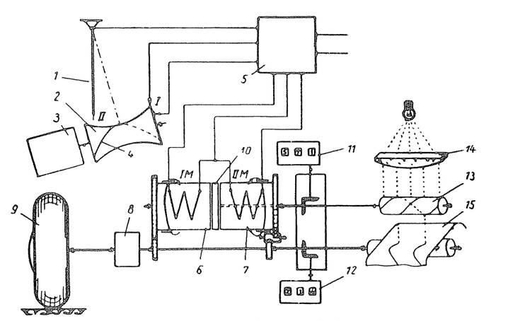
Figure 22 : Schematic of components of WA-1M Automatic Altimeter.
In April 1961, the United States Geological Survey took delivery of two Johnson Ground Elevation Meters (JGEM, sometimes just GEM)(Speert, 1962). During his 1963 visit to the United States, Bruce Lambert Nat Map’s Director, saw a demonstration of the Johnson Ground Elevation Meter and along with the Royal Australian Survey Corps, two were ordered for Australia. Nat Map’s JGEM was delivered in August 1964, and accepted after tests at Balcombe in Victoria, in conjunction with the RA Survey’s vehicle. Figure 23 shows a photograph of Nat Map’s JGEM.
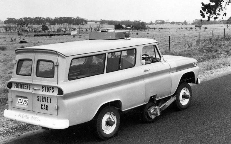
Figure 23 : National Mapping’s Johnson Ground Elevation Meter.
The Sperry Sun Well Surveying Company, not Sperry Rand as in some literature, manufactured JGEM was a highly modified General Motors Corporation truck having 4 wheel drive and simultaneous front and rear steering. Using a very sensitive pendulum and a fifth bogey wheel the difference in height was determined using the principle of the sine of the inclination of the vehicle multiplied by the distance run. The JGEM’s specifications were developed by the United States Department of the Interior, Geological Survey, Topographic Division. These specifications came from many years of use of the 1952 trailer mounted version of the equipment. Please refer to Figure 24 below.
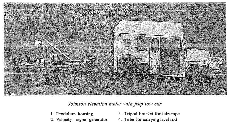
Figure 24 : Trailer version of the Johnson Ground Elevation Meter (best photo quality available).
As the fifth wheel required a relatively smooth surface to maintain accuracy, the quality of Australia’s roads did not allow maximum accuracy to be achieved. Nevertheless, National Mapping did obtain results with an error of less than 10 feet (3 metres) in 50 miles (80 kilometres) at 15 miles an hour (25kph) on reasonably good road surfaces, averaging 100 miles (160km) per day. Overall, between 1964 and 1970, around 5% of all National Mapping vertical control was obtained using the Johnson Ground Elevation Meter. In flat country, where the sealed road system was reasonably extensive, the JGEM demonstrated that a network of heights could be obtained which would allow contouring for 1: 100,000 scale mapping from 1: 80,000 scale aerial photography. Contours in photogrammetric blocks 3 and 4 in Queensland, block 18 on the Victoria/New South Wales border and part of block 32 in New South Wales were plotted from heights obtained by JGEM traverses. For their part, RA Survey used their JGEM to obtain height information within some fifteen 1: 250,000 scale map sheets. The Photogrammetric Blocks which used heights obtained by the Johnson Ground Elevation Meter to provide vertical control for mapping are shown in Figure 25 below.
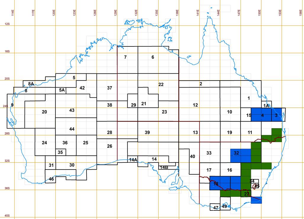
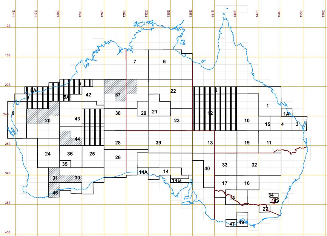
Figure 25 : Photogrammetric Blocks which used heights obtained by Nat Map’s Johnson Ground Elevation Meter to provide vertical control for mapping are shown in blue; green areas are where RA Survey used their JGEM.
As well as being used to obtain vertical mapping control points, Nat Map’s JGEM was applied to two other tasks where reasonably accurate elevation data were required. One such task was to obtain longitudinal height profiles of a number of airstrips, mainly in outback Queensland and New South Wales. A consistent height datum for each airstrip profile was obtained by a connection to the nearest Bench Mark. These profiles were used in the calibration of the radar based Airborne Profile Recorder system. The other task was to provide check heights to ensure that the contractor’s APR heights were to an acceptable accuracy.
While height acquisition by vehicle was faster than traditional levelling, its areas of operation in Australia were extremely limited and for the majority of Australia’s then outback, entirely unsuitable.
Chapter 3 - Evolution of Airborne Vertical Control Acquisition
Vertical Control by Radio Altimeter
To assist with the compilation of aeronautical navigation charts in remote parts of Canada, its National Research Council investigated a means of obtaining airborne terrain profiles. Experiments with airborne altimetric measuring instruments thus began around 1946. The APN-1 radio altimeter, as shown in Figure 26 below, had been designed to be installed in aircraft to provide direct measurement of altitude relative to the terrain during flight. A transmit and receive antenna were mounted on each side of the fuselage with the frequency difference between the transmitted and received signal being converted to the aircraft to ground distance or height above terrain. This value was conveyed to the pilot via a cockpit mounted meter. Height above terrain however, was limited to 4000 feet with the APN-1 and its testing proved that specifically designed equipment was needed to acquire height data from an airborne platform over extensive areas.
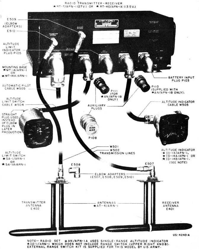
Figure 26 : Configuration of an APN-1 Radio Altimeter showing cockpit instrumentation and transmit and receive antennae.
An airborne pulsed radar instrument was designed, which by 1947 was giving terrain profiles to an accuracy of 200 feet. This accuracy was adequate for the Canadian’s purpose as the required contour interval was 500 feet.
In his 1948 report A Pressure-height Corrector for Radar Altimetry, McCaffrey of the National Research Council, Canada, stated that…in order to compensate for deviation in height - it is impossible to maintain constant height over long periods - pressure altimeters have been photographed at the rate of 1000 to 2000 times per hour during flight. Data so obtained has been used to correct the radar graph to the nominal operating height with an accuracy of perhaps ten to fifteen feet.
McCaffrey’s report went on to describe a new datum stabiliser using a Hollsman type altimeter. This was successful but was later superseded by the Hypsometer using the boiling point of toluene to detect pressure changes.
The Hypsometer thus became an essential element of the terrain profiler system, essentially monitoring the airborne datum during terrain profiling operations. The airborne datum was the aircraft altitude, but as aircraft altitude is measured by the change in atmospheric pressure, the airborne datum was actually a pressure surface. Maintaining a constant flight level required maintaining a constant pressure or isobaric surface. As precisely following this surface was impractical, the approach was the measurement of any departure from a set altitude and later make the necessary corrections. At profiling altitude, the atmospheric pressure at that height became the reference sample and throughout profiling operations any deviation in height and therefore pressure was measured and recorded. The deviations could then be used to adjust the radar terrain profile. As the deviations were relatively small, generally less than ±100 feet, their magnitude could be measured to a high accuracy.
This accuracy was achieved by using the boiling point of toluene to detect pressure changes. Inside the Hypsometer, a vessel of liquid toluene was kept boiling by resistors. A sensing element mounted above the boiling toluene formed one side of a bridge circuit; the other side of the bridge was continually balanced by a servo operated potentiometer in the Hypsometer chassis. An outside pressure change meant that to keep the bridge balanced extra electrical current had to be supplied to the circuit. This additional electrical current was electronically converted to a change in height and applied to the measured terrain clearance to give the terrain profile. The terrain profile then being the record as referred to the selected initial flying height or isobaric surface. The change in height as measured by the Hypsometer was not directly recorded but could be deduced from the difference between terrain clearance profile and the terrain profile at any given point.
The Photographic Survey Corporation (PSC) Limited of Toronto, developed similar equipment for commercial use. Speert (1950) stated that in 1950 the United States Geological Survey (USGS) undertook what is believed to be the first attempt in the United States to obtain ground elevations for topographic mapping by airborne electronic methods. The work was done under contract, by Photographic Survey Corporation, Limited, of Toronto, Canada, and its affiliated company, Kenting Aviation, Limited, using the Airborne Profile Recorder (APR). Approximately 78,000 square miles in central Alaska were covered on this project. Of 29 control elevations examined in the reconnaissance portion of the project, only one feature exceeded the allowable spread of 30 feet. Four runs over this feature showed height values with a total spread of 44 feet, but three of the values fell within a spread of 24 feet. One reading was obviously bad. Except for this feature, the maximum spread was 26 feet, and the average spread was 14 feet. Unfortunately, there were no opportunities to check the absolute elevations of any of the control features in this area.
By 1955, the Airborne Profile Recorder (APR Mark IV) was refined enough to give accuracies of ±15 feet and around 1959 the Mark V APR was introduced, which was relatively smaller and lighter with an accuracy of ±10 feet. The Canadian Applied Research Limited (CARL) Mark V, radar profiler was able to operate from 1,500 to 45,000 feet and measured the aircraft to ground distance. The 3 centimetre band radar beam was radiated at 2000 Hertz and projected in about a 1° cone from an antenna in the centre of a 44 inch (1.1 metre) parabolic reflector. This reflector was mounted to point directly below the aircraft such that an area with a radius of about 55 meters on the ground would be illuminated from a normal operating altitude of about 10,000 feet above sea level.
The earliest radar profiler trials used an F24 camera adapted to 35mm strip film for the positioning camera because no commercial camera was available. This led to the later development of the CARL 35mm positioning camera, and associated controls as used on the CARL Mark V APR. Camera magazines held 400 feet of 35mm film and lenses of 90mm or 28mm focal length could be used. Controlling the positioning camera’s rate of exposure was an intervalometer. The axis of this camera, marked by the cross in the image, was directed down the axis of the radar reflector. For accuracy, it was critical that the vertical axes of the radar antenna and positioning camera were collinear.
A few lines on page 25 of the Ottawa Citizen newspaper of Wednesday 19 November, 1958, stated that the Canadian designed and built Airborne Profile Recorder (radar surveying unit) has been selected by the USAF for its massive, program of bringing the world's geography up to date…The Recorder is made by Canadian Applied Research Limited, a company owned by A.V. Roe (Canada) Limited. Annexure D provides an overview of PSC’s development. Starting with PSC’s foundation to its ownership by AV Roe (Canada) Limited, a wholly owned subsidiary of Hawker Siddeley, and later integration with de Havilland Canada’s Special Products division to form SPAR (Special Products and Applied Research) Aerospace Limited, to today being a part of MacDonald Dettwiler as MD Robotics, a subsidiary of its MDA Space Missions division. The overview concludes with MDA’s association with National Mapping’s, Australian Landsat Station (ALS) and later Australian Centre for Remote Sensing (ACRES).
The USAF adoption of the APR appears to have resulted in its satisfactory performance in tests conducted in the United States as reported in the 1961 paper, Investigation of the Air-Borne Profile Recorder, by Chester Slama of the US Army Map Service (Slama, 1961).
Vertical Control by an Airborne Profile Recorder
The Airborne Profile Recorder (APR) Mark V, was made by the then Canadian Applied Research Limited (CARL), a company owned by AV Roe (Canada) Limited, which in turn was a wholly owned subsidiary of Hawker Siddeley.
The CARL Mark V, APR radar transmitter/receiver, 35mm positioning camera, Hypsometer and associated graphical chart recorder, power supply and controllers were combined into three major components for aircraft installation. Figure 27 below shows this instrumentation prior to installation in an aircraft.
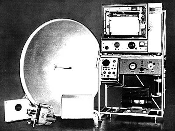
Figure 27 : Canadian Applied Research Limited (CARL), Mark V, Airborne Profile Recorder instrumentation.
The radar reflector is left with 35mm camera in foreground and operator’s console right.
The radar’s parabolic reflector was mounted to point directly below the aircraft. The 35mm positioning camera was rigidly mounted to the reflector assembly so that the optical centre of the camera was in alignment with the beam centre of the antenna. Electronics controlling the radar’s transmitter-receiver was mounted close to the antenna. This equipment weighted some 50lbs.
The size of the antenna and reflector in this system provided a 1° cone of the transmitted signals at the point of emission. At an operating altitude of 3000 metres these signals sampled a circular area of the terrain some 55 metres in diameter. To reduce the sampled area a much larger transmitter reflector would have been required and this was not considered practicable.
The operator’s console, as shown in Figure 28 below, was mounted in the aircraft cabin. It contained the graphical chart recorder and its controls at the top, with power panel below. Camera intervalometer and frame counter below that and near the base an inverter and the Hypsometer. A total weight of about 100lbs.
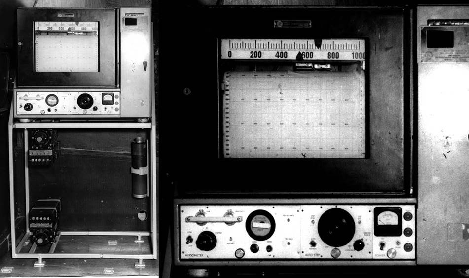
Figure 28 : Photograph (left) of the APR operator’s console as mounted in the aircraft cabin where below the graphical chart recorder, inverters and the Hypsometer can be seen.
The enlargement (right) shows the graphical chart recorder and paper chart.
The inverter converted the aircraft power supply from 28V DC, to 115V AC at 400Hz for the powering the APR system controlled by the power panel. The Hypsometer was connected to a pitot tube which conveyed outside pressure changes via a static line. A graduated dial (±150 feet range) on the hypsometer panel gave the operator an indication of height above or below the isobaric surface, and a repeat instrument was mounted to the right of the pilot to enable him to control aircraft height. Throughout the profiling operation the aim was to keep the aircraft as close to the selected isobaric surface as possible by keeping the Hypsometer gauge reading as close to zero as possible and certainly not outside the ±150 feet range. Many miles of profiling were hand flown by the pilot until automatic pilots (autopilot) became accurate and cost effective. While the autopilot then reduced the size of the aircraft’s departures from the isobaric surface, these instruments did not negate them totally.
The graphical chart recorder provided the permanent record of terrain profiling operations. The dual (red and blue) pen recorder was mounted on a hinged assembly which opened like a door to permit chart changes and inspections. Chart rolls were about 122 feet long and exactly 12 inches wide. Margins for the chart drive sprockets used 1", leaving 11" to record the outputs. A blank chart looked like a long roll of graph paper having a lightly printed grid. The grid itself was not really used other than the first printed line above the sprocket holes which became the chart datum. This line rather than the very first printed line was adopted as it was unlikely to be affected by any tearing, uneven rolling or mishandling of the chart. The vertical scale was set at 1.1 inches to 100 feet thus permitting a 1,000 feet rise or fall to be recorded. The horizontal scale was variable, since aircraft ground speed varied, but was around 1,250 feet per inch. The chart moved at 10 inches per minute (ipm) but could be varied from 5-20ipm in 5ipm increments. A servo motor actuated the red and blue pens across (left/right direction during recording) the chart to depict the terrain profile (red) and terrain clearance (blue) traces. The difference between the two traces gave the Hypsometer reading, which could be checked visually against the Hypsometer gauge. On the right hand edge of the chart a third pen recorded the positioning camera exposures. As the ink traces on the chart were the only record, maintenance of the operation and pen sensitivity was critical. Figure 29 below, shows an example of an APR chart and associated 35mm film.
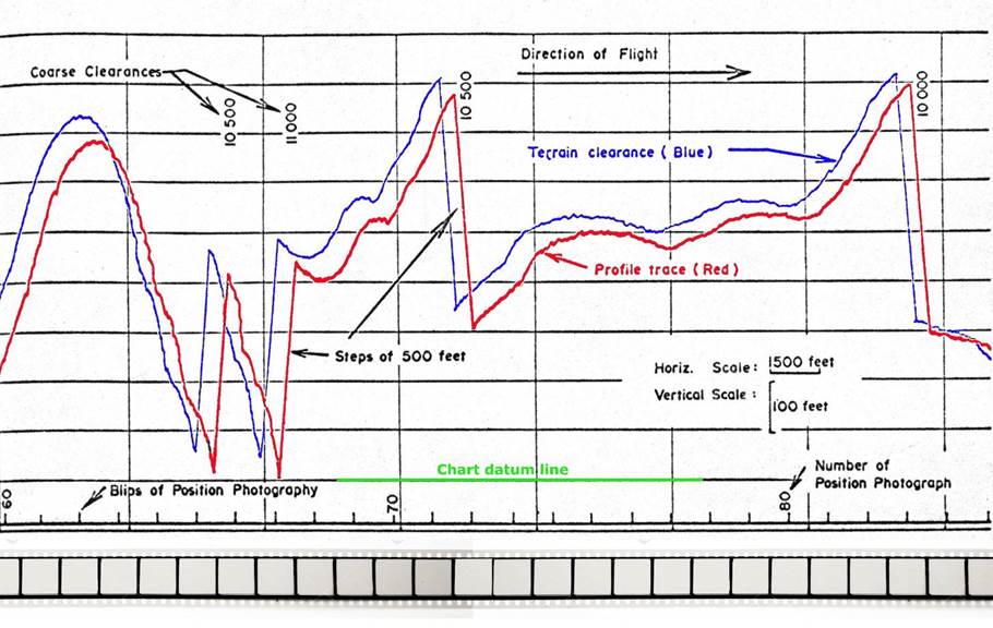
Figure 29 : Example of an APR chart and associated 35mm film.
The terrain profile is the red trace and the location in the terrain is established by the 35mm positioning photography which is related to the chart by the blip made at the instant of each exposure.
The autostep could be operated either manually or electrically. The coarse range reading was shown on a dial marked from 1 to 20.5 (x 1,000 feet). A manual coarse range control from 0, 5, 10, 15, 20 (x 1,000 feet) enabled the operator to adjust the coarse range setting. The sum of the coarse range and step range dials were recorded on the chart by the operator and which, when added to the height indicated by the pens, gave the total height above the terrain.
The radar system was pulsed at a rate of about 2,000 pulses per second, and the echo delay time went to a quartz crystal controlled oscillator for maintaining precision of measurement. The terrain profile drawn on the chart was thus the result of a sampling of statistically derived groups of measurements. This approach smoothed out excessive noise in the profile and provided a better and more usable trace.
While not part of the APR equipment itself, a necessary requirement for profiling was a drift sight or drift meter. Such a sight was an optical instrument which allowed the terrain below the aircraft to be viewed from inside the cabin; it can be thought of as a periscope in reverse. It was used in aircraft navigation for determination of drift and to ensure the aircraft flew along a precise section of the terrain. Its design allowed it to be rotated through 360° and the rotation could be measured on a scale; 0° / 180° on the scale was generally aligned parallel with the aircraft’s centreline. Drift was determined by following an object in the terrain and to make the object appear to move parallel to the sight’s reticule lines by carefully rotating the sight. The amount of rotation, estimated to ¼°, from 0° was the aircraft’s drift. The drift sight can be seen in Figure 30, just to the left of the operator’s console, near the window.
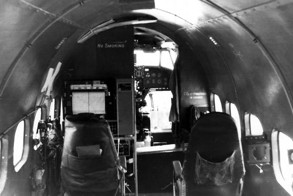
Figure 30 : Photograph of the APR operator’s console as mounted in the aircraft cabin of an ADASTRA Hudson.
Just to the left of the console, near the window, is the drift sight (Photograph courtesy Owen Smith).
The Isobaric Surface as a Datum for Airborne Terrain Profiling
Maintaining a constant flight level during terrain profiling operations required maintaining a surface of constant pressure. Such a surface is known as an isobaric surface where the atmospheric pressure is equal at every point.
An isobaric surface is generally curved, and although a small part can be considered a plane it is never horizontal. There are also diurnal variations in its altitude. The altitude of the isobaric surface above sea level depends upon the density, and hence the temperature, of the intervening air column. In regions where the air in that column is cold and dense, the altitude of that isobaric surface will be lower than over a region where the air is warmer and less dense.
TJG Henry of the Meteorological Division, Department of Transport of Canada in 1947 determined that the slope of an isobaric surface could be calculated and this calculation became known as the Henry correction. Annexure E contains more detail and shows that the Henry correction is proportional to the sine of the drift angle times distance flown.
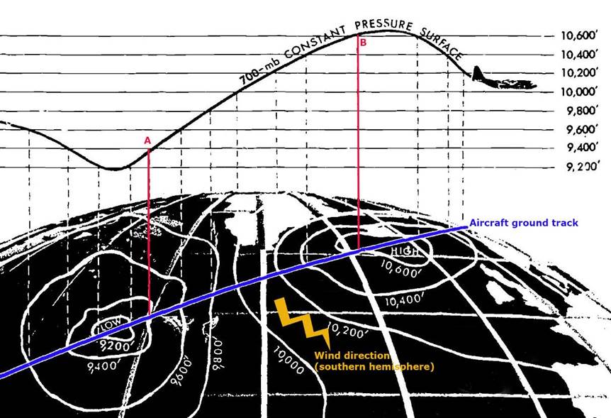
Figure 31 : Diagrammatic view of the Henry Correction for the southern hemisphere.
In summary, Henry found that in the southern hemisphere (for the northern hemisphere the results are reversed) that an aircraft flying from a low pressure to high pressure region will drift to the right or starboard, incurring starboard drift. In these same conditions, if the aircraft maintains a constant pressure altitude, that is it flies an isobaric surface, it will fly a path above the theoretical surface. Thus, with starboard drift the height correction needed, actual to theoretical, is positive. Conversely with port drift, the sign of the Henry correction is negative in the southern hemisphere. Figure 31 above diagrammatically shows a line A to B being flown and the atmospheric pressures at the time of flight. In these conditions, if at position A, the reference pressure of 700 millibar was captured and that 700 millibar pressure surface was precisely maintained by the aircraft to point B, then the isobaric surface has risen by 1,200 feet (10,600 minus 9,400 feet) above the theoretical surface. In theory, the Henry correction for this flight would be found to be around +1,200 feet. From Figure 31 it can also be seen that the reverse is true if the line B to A was flown. If the 700 millibar pressure surface had been captured at point B then at point A the Henry correction would theoretically be -1,200 feet.
It is very important to note that in this example the value for the Henry correction is simply applied in relation to the theoretical surface. Assume now that points A and B in Figure 27 are at sea level. The terrain clearance, aircraft to ground distance, would be 9,400 feet at A and 10,600 feet at B. If the reference altitude of 9,400 feet at A was taken to have been maintained to point B, then the height of point B would be calculated from reference altitude minus terrain clearance measured at point B (9,400 minus 10,600 feet) giving -1,200 feet as the height of point B. Clearly to get the correct height at point B the value for the terrain clearance at point B has to be reduced by the value found for the Henry correction. That is, reference altitude minus terrain clearance measured at point B reduced by the value of the Henry correction at point B (9,400 minus (10,600 minus 1,200) feet) now giving the correct value of zero feet. This example demonstrates why in some literature the sign of the Henry correction is reversed when that correction is made to the terrain clearance distance.
Thus, on any airborne terrain profiling operation, the slope of the isobaric surface was the Henry correction divided by distance flown and this value could be found by monitoring aircraft drift and calculating the distance flown, as described in Annexure E. With the slope of the isobaric surface calculated, the required level surface could be redefined at any point during profiling. In the southern hemisphere, to derive the correct sign (±) for the Henry correction the sign (±) for the determined amount of port drift is negative and conversely the sign (±) for the determined amount of starboard drift is positive.
Henry’s work on the theory of pressure pattern determination from drift measurements, was an advancement of that by Dr John C Bellamy (United States Air Force) in 1943. Bellamy developed a procedure for determining a close approximation to the beam wind component, that is the force of the wind acting on the aircraft and affecting its course. Using the geostrophic assumption and pressure measurements made at an aircraft’s altitude with radio and pressure altimeters, the drift angle calculated by this method of navigation was known as Bellamy Drift.
Operational use of the Henry Correction
Mathematically modelling the atmosphere via Henry’s method was useful but all the real world variabilities could not be included is such a simple correction. Airborne terrain profiling operations were such that lots of small factors could accumulate and effect the final accuracy of the derived terrain heights. An operational procedure was thus developed which would account for any residual errors and refine the final terrain heights.
The procedure was to overfly a datum surface after takeoff and at profiling height, and while still at profiling height, overfly a datum surface before landing. While the datum surface was usually the same place, operationally it could be two different locations. Without these datum runs an operational flight could not yield reliable data. The size of the radar beam as it was reflected from the terrain demanded that such a datum surface be of significant size and its surface relatively plane. Further, the height of this surface needed to be found using a suitably accurate traditional survey method. Airfields, lakes or a calm sea thus became the most suitable sites for use as datum surfaces. In Australia, airfields became the datum surface of choice and the specific one that was being used as the operational base for the airborne operations generally became the datum surface.
To provide the necessary datum information any airfield used as a datum surface generally had the centreline(s) of its strip(s) levelled and connected to the Australian Height Datum (AHD). As the area around airstrip intersection(s) and/or the windsock could be easily identified on the positioning photography, heights of features in these areas were acquired as well.
After takeoff, the profiling aircraft would climb to operating altitude. Here the reference sample of air would be captured by the Hypsometer. With all equipment operational and initial drift found, the centreline of the airfield would be overflown. The airfield’s profile was recorded on the chart and the profile’s position by the 35mm camera. The aircraft would then navigate to the profiling area. During this time there was no need to run the profiler or camera but maintaining height with reference to the Hypsometer and the recording of air speed and drift were vital for later Henry correction computation. After completing the required terrain profiles and recording the navigation data on the return to base, the centreline of the airfield would again be profiled with the profiler and camera running. The aircraft would then land.
While the chart recorder and camera only needed to record the necessary profiles, it was critical that the Hypsometer be operational from the after takeoff datum overfly until after the prelanding datum overfly. During this same period of the flight, the pilot had to maintain the aircraft in close proximity to the isobaric surface as shown on his Hypsometer repeater. Any failure/problem with any one of these aspects could render the whole flight meaningless.
To validate a profiling flight, the Henry correction would be calculated for each section of the flight where the drift was constant. The mathematical sum of the Henry correction for each section of the flight, gave the total Henry correction for that flight. As the Henry correction at the after takeoff overfly was zero, the elevation of the airfield plus the height of the aircraft above the airfield, as given by the profile on the chart, gave the height of the isobaric surface on AHD. At the prelanding overfly, the elevation of the airfield plus the height of the aircraft above the airfield, was similarly calculated. However, this height had then to be corrected by total Henry Correction for the flight. In theory, this final value should have given the same height for the isobaric surface as at the start, but invariably there was a residual. As this residual accumulated as the flight progressed it could be proportioned per unit of distance flown.
Operationally therefore, the terrain heights extracted from the terrain profiles were not only corrected for the slope of the isobaric surface, but also for a residual which accounted for the myriad of other small variables which otherwise impacted final accuracy.
Part 2 - National Mapping’s use of Airborne Terrain Profiling for Vertical Control Acquisition
Chapter 4 - Contract Airborne Profiling
CARL Mark V Airborne Profile Recorder (APR)
Based on the experience of overseas agencies with APN-1 radio altimeter equipment, National Mapping’s then sister division, the Bureau of Mineral Resources, used surplus wartime APN-1 equipment on some of its airborne geophysical work. While not really suited for the airborne heighting of vast areas, as had also been discovered overseas, this equipment seemed the only option at the time for Nat Map to pursue in an attempt to speed up its acquisition of height data. Surplus APN-1 equipment was thus purchased by Nat Map in 1962, and tests using the radio altimeter in a light aircraft were planned (Lines, 1992). Before the testing commenced however, Nat Map learned that another option had just become available.
Adastra Airways, an Australian pioneer in the commercial aerial photography market, had procured a Canadian Applied Research Limited, Mark V, airborne profile recorder and installed it in a Lockheed Hudson. The Hudson’s bomb bay made an ideal location for the installation of the 1.1 metre diameter radar antenna reflector. To retain the aircraft’s aerodynamic lines, the original bomb bay doors were modified and partially replaced by a fibreglass cover. This option of heighting by airborne profiling was far more attractive to National Mapping, thus the APN-1 tests were hastily abandoned in favour of a trial contract with Adastra Airways for radar terrain profiles with its CARL Mark V APR. The contract was fulfilled later in 1962 in the Mount Coolon-Clermont area of Queensland where the Government was encouraging natural resources development, and required topographic map coverage (Lines, 1992).
Shute (2016) described the Adastra installation and operations. The Mark V radar profiler was fitted to Adastra’s Lockheed Hudson’s VH-AGX, VH-AGS and VH-AGJ at various times. Please refer to Figure 32 below. The equipment consisted of a radar reflector inside the bomb bay directed vertically downwards through a circular cutout in the bomb doors. This aperture was covered externally by a removable fibreglass panel.
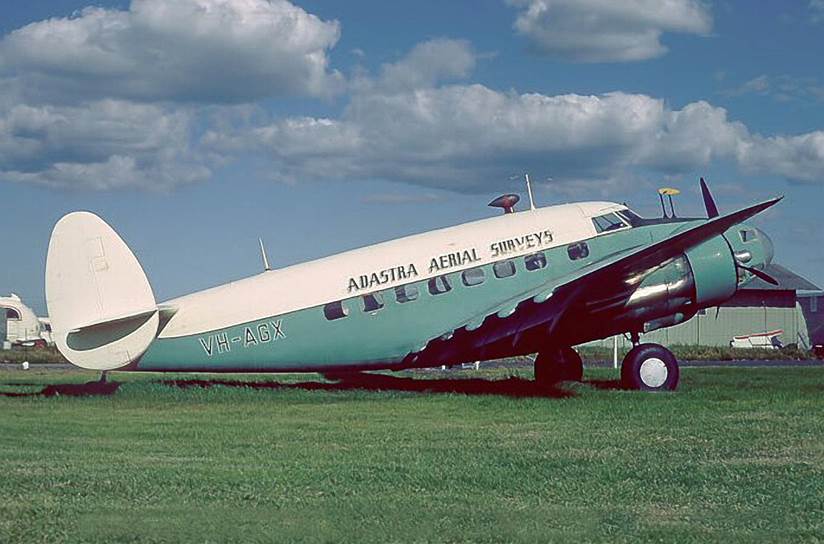
Figure 32 : ADASTRA Lockheed Hudson VH-AGX (Photograph courtesy Owen Smith).
The technician's
equipment in the aircraft was set up on the port side of the main cabin, immediately
behind the forward bulkhead. All the electronic gear (valves in those days), with
an oscilloscope was set up on Dexion shelving, and was about five feet high by
four wide. In the centre, facing the technician was the continuous rolling
chart on which a pen marked a line showing the profile of the ground directly
underneath the aircraft. The centre line of the chart represented the datum
height. The 35mm positioning camera pointed down through the floor on the
starboard side of the bomb bay, next to the reflector and had its own access
panel for changing film and settings in flight.
As the radar profiles were to provide height data to control previously acquired aerial photography the required profile flight lines were usually drawn on a series of these photographs that had been taped together to form a long roll.
Navigation was carried out using a standard drift sight that protruded through the floor just aft of the nose Perspex. This had a graticule along the fore/aft axis and a prism under the instrument that could be tilted to give a view anywhere from the forward horizon to just aft of the vertical. With a vertical view of the ground beneath drift was ascertained. Profiling was carried out from an altitude of 10,000 feet and once at operating height a drift reading on a heading appropriate to the datum airstrip was taken. The aircraft had to be flown, as accurately as possible, down the centre line of the airstrip for a datum check to be made. This could be the base strip or another in the area, the ground profile of which was already known from ground survey. The equipment would be running on the lead up to the runway and at the start of the runway overfly the technician would mark the chart accordingly. At the end of the runway overfly, the chart would be marked again. From the time that the initial datum run was started, until such time that a similar procedure was carried out at the end of the sortie, the time at each new heading or drift change had to be logged.
Once a recognizable profile of the strip had been recorded, the aircraft was navigated to the first profile flight line. The chart would be marked at the beginning of the profile and from then on it was a case of navigating the aircraft as close as possible to the flight lines drawn on the aerial photos or map. Drift would be checked periodically and heading corrections made as required. At the end of the profile line the chart was again annotated.
The autopilot on the Hudson was very stable and, if the conditions were right, long distances could be covered without any corrections being made. Heading corrections were kept as small as possible and were usually of one or two degrees, which just needed a touch of the autopilot knob. The main problem with profiling work was turbulence, which could build up very quickly in the remote areas and many flights were cut short because of it, as a change in attitude would give false profile readings on the chart. The final run over the datum airstrip at the end of the sortie had to be as accurate as the first and in bumpy conditions it was sometimes quite tricky for everyone. Without it however, all would be wasted.
Survey flight times could be anything up to six hours on a good day but the norm was usually about four.
Between 1962 and 1973, it is understood that Nat Map let some nine separate contracts to Adastra to provide radar terrain profiles over specific blocks of 1: 250,000 scale map sheets. In its simplest configuration a block consisted of a single profile area equivalent to a 1: 250,000 scale map sheet covered by eight strips of aerial photography. Due to terrain height some areas required nine strips of aerial photography in which case extra profile lines would have been flown. Assuming that no profile lines had been flown in the map areas surrounding the map area to be profiled, nine east-west profile lines were necessary in the aerial photography’s side overlap as well as north-south tie lines at each degree of longitude and map sheet extents amounting to a further three profile lines. An example of the positioning of APR flight lines along the lateral overlap of successive strips of aerial photography is shown in Figure 33 below. Figure 34 below shows an example of the profile lines and their approximate position for a standard 1: 250,000 scale map sheet of 8 strips of aerial photography.
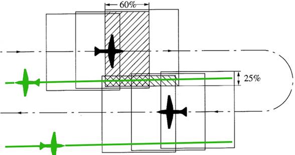
Figure 33 : Example of APR flight line positioning in aerial photography sidelap.

Figure 34 : Example of the APR flight lines required for a standard 1: 250,000 scale map sheet of 8 strips of aerial photography.
Profiling contract blocks were generally multiple adjacent 1:250,000 map sheet areas. Thus, if practical, east-west lines were extended as when profiling once on line it was more efficient to maintain the line. Likewise, north-south ties extended the length of the contract block.
As part of the tender process, the Contractor was asked to provide the following certifications as a minimum :
|
- |
appropriate Airworthiness certificate(s) for the aircraft to be used, with approvals to undertake the profiling work; |
|
- |
that modifications to the aircraft necessary for the equipment’s installation and operation had been approved; |
|
- |
that the radar range had been calibrated; |
|
- |
that the axis of the positioning camera had been aligned with, or is parallel to, the axis of the radar beam; the alignment would also be required to be checked and certified on completion of the work; |
|
- |
that instruments like the air speed indicator, compass and outside air temperature gauge had been calibrated and current correction information was readily available to the crew during a flight. |
Payment was usually made on receipt of deliverables from the Contractor, the timing of which would be agreed with the Contractor. Such deliverables usually included :
|
- |
charts and films, uniquely labelled and identified as specified; |
|
- |
the annotated charts containing the following : - the clearance trace (in blue); - the profile trace (in red); - a Hypsometer sensitivity check (undertaken at operational altitude and before the after takeoff datum run, to ensure the Hypsometer was functioning correctly and any pressure change was being accurately recorded. The aircraft was thus made to climb and descend about 150 feet which resulted in the profile trace (red) to trace an almost horizontal line while the clearance pen (blue) showed a sinusoidal trace reflecting the aircraft’s movement). - the position camera trace (the horizontal line generally located along the bottom edge of the chart with sudden deflections or blips corresponding to each exposure of the positioning camera; at regular intervals the chart was annotated with the corresponding frame number shown on the camera’s frame counter): - change of datum (when either the clearance trace or profile trace approached the edge of the chart the technician could, automatically or manually, deflect both pens by a constant amount either upwards or downwards to prevent the pens from running off the chart; the value of this change of datum was annotated on the chart); - the pen calibration (recorded at the beginning and end of each flight, the relative positions of the red and blue pens, which were offset so they could move freely and independently across the chart, was recorded; while the chart was stationary the pens were made to draw vertical lines, Nat Map required that the blue pen be offset so that the red pen’s position, which was accurately recording the terrain, was centred in the frame of the positioning photograph); - datum profiles (required at the start and end of each flight). |
|
- |
rolls of processed 35mm negatives and rolls of corresponding, printed positioning photographs; |
|
- |
flight logs containing times of heading or drift changes, start and end of profiling, crossing of significant features as well as altitude, indicated air speed, outside air temperature, positioning camera and chart settings; |
|
- |
a diagram at 1: 250,000 scale, showing the complete flight details for all lines profiled (this plot allowed the distances flown to be scaled for use in the Henry correction); |
|
- |
the Contractor’s Henry correction calculations for each flight showing that the flight met the required accuracy standard (National Mapping required that the value for the Henry correction not exceed ±50 feet for a flight to be acceptable under the contract); |
|
- |
calibration data to permit air speed indicator, compass and outside air temperature readings to be corrected before being used to check the Contractor’s Henry correction computations. (Essential to the Henry correction was True Air Speed (TAS) which was calculated from the indicated air speed (IAS) readings, corrected for the outside air temperature (OAT). Before TAS was calculated however, the IAS and/or OAT instrument readings were adjusted according to their respective calibration data). |
When a radar terrain profiling contract was let, National Mapping supplied the Contractor with a series of 4 digit line numbers to be allocated to each profile line as it was flown. The allocation of such numbers was carefully administered to ensure that no number was used more than once. At the end of the contract the Contractor had the responsibility of specifically advising on the line numbers used thus allowing unused numbers to be reallocated. As had been the practice in the past with survey stations and aerial film numbers, the state alphabetic identifier formed part of the profile line (APR) identifier (B-Queensland, C-New South Wales, D-Victoria, E-South Australia, F-Western Australia, G-Northern Territory). Any terrain profile flown along a state border incorporated the state codes of both states. For example, a Western Australia profile line might be identified as APR/F/2345, a Victorian profile line as APR/D/1357 and a profile line along the Queensland-South Australia border as APR/BE/1789. This unique identification system later allowed the contractor supplied profile materials to be registered, stored and retrieved on demand.
On receipt of a batch of deliverables from the Contractor by Nat Map, and after careful checking that what the Contractor listed as being sent was indeed sent, the materials were registered and boxed for storage. It was found that boxes the size of a shoe box was able to contain the chart and films, negative and print, for a single terrain profile. Each such shoe box was given a unique 3 digit number in sequence, which was stencilled on the front of the box so it could be easily seen when the boxes were stacked on shelves. Each shoe box was then filled with the chart and films for a specific profile line. Pages of a ledger were prepared listing in sequence the series of 4 digit numbers supplied to the Contractor. When the profile data was received, the number of the relevant shoe box containing the profile data was then entered in the next column. Other columns, listed information like contract number, profile and delivery dates. The logs and calculations were generally filed in folders labelled with the contract number and delivery date. At the end of a contract unused line numbers in the ledger would have no other entry and would be left blank in case at some later time the line number was used.
When work was then required on a specific profile line it was a simple matter of scanning down the ledger pages for the APR line number, finding the associated shoe box number and retrieving that box from the storage area. The shoe boxes kept the materials together even as they were being worked on and it was very rare for materials to get mixed up or lost.
Before payment was made to the Contractor, Nat Map independently checked the Henry corrections for each profile line. In the early days, with most staff out of the office on field work for a large part of the year and then having to take leave on their return, there was hardly anyone for this computational work. Nat Map was reluctant to pay for possible inaccurate work but the Contractor wanted payment and there was some discord. It was especially difficult when Nat Map wanted lines to be reprofiled as the initial profile was deemed not to meet specifications. By this time the Contractor was generally well out of the area on some other work and repositioning costs became a point of tension. Fault on both sides saw letters back and forth with, especially in later years, intransigence as another driver for Nat Map to obtain its own system. As will be seen, Nat Map then used its own more accurate laser profiler to reinforce the radar profiling, when required.
Figure 35 shows where terrain profiles were obtained by ADASTRA with their CARL APR system, under contract to Nat Map.
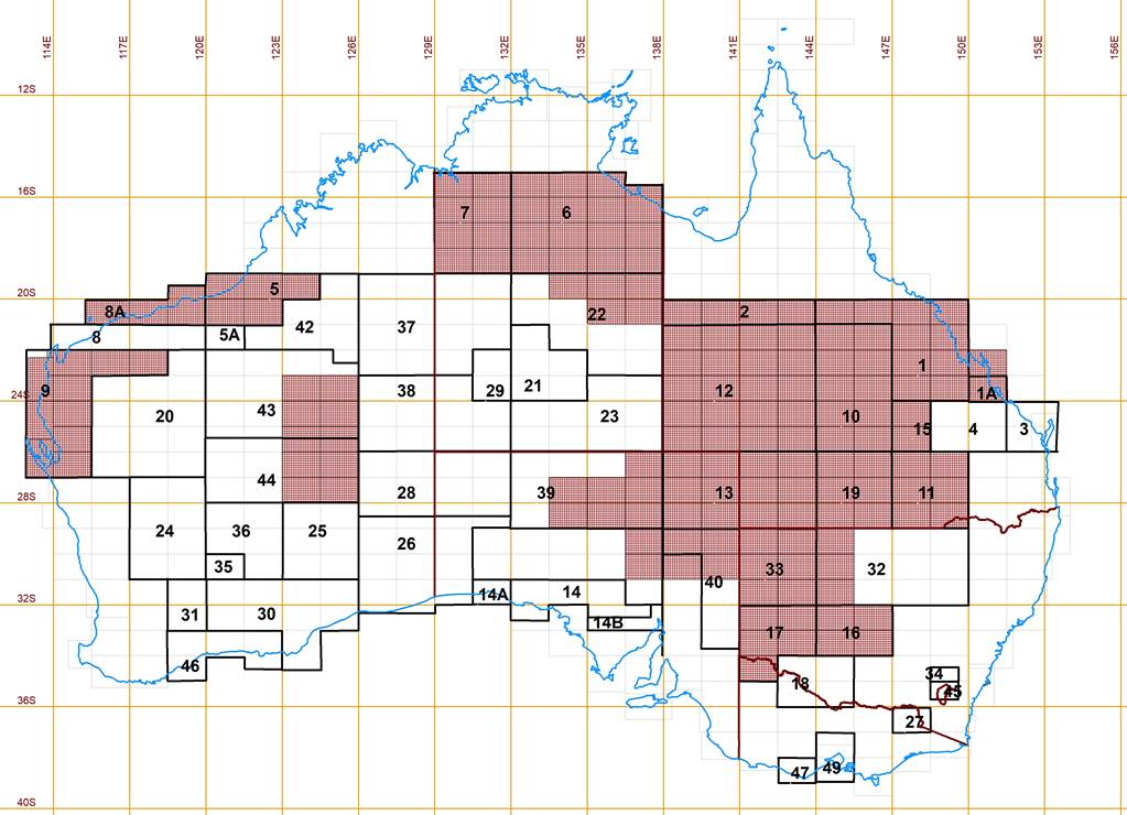
Figure 35 : Map showing the 1: 250,000 scale map areas where contract APR was completed by ADASTRA for Nat Map.
Extracting Vertical Control from CARL Mark V, APR Terrain Profiles
In parallel with the slotted template adjustment of the photogrammetric block the necessary terrain heights were extracted from the radar terrain profiles. The photogrammetric models from which the map detail would be ultimately plotted had been determined earlier for use in the slotted template adjustment. This meant that the general locations for height control in each photogrammetric model corner were defined and the APR positioning photography should also cross that area. Sequentially, using features identified in both the photogrammetric models and the APR positioning photography identical points were marked in the model’s overlap and numbered on both sets of photography. Where possible the location of the principle point of the APR positioning photoframe, which was shown in each frame by a cross, was transferred to the model. However, any location along the positioning photography’s flight line could be used as it was possible to accurately interpolate between positioning photocentre blips on the chart.
At least two points would be selected in each corner location of the model, such that the point’s locations were on the most open and flattest terrain. The two points acted as a check against each other and selecting them on open, flat terrain gave the best height accuracy of the radar system given its wide sampling area. If the points’ locations were other than optimal, more points would be selected to give options to the photogrammetric operator when setting up the model for plotting. In say a group of four points the operator may find that two of the four points enabled better model orientation and so these could be used. As photogrammetric plotting might take place months after height extraction it was better to select and compute the heights of a few more points at this time rather than to have to come back at some later time and generate more control points. Nevertheless, this did happen from time to time.
As a precursor to extracting heights from the radar profiles for a 1: 250,000 scale map sheet some preliminary computations were undertaken to validate the vertical integrity of the APR profile lines.
Using the positioning photography, the intersections of each east-west profile line with the three north-south profiles would be found. Heights for each of these intersection points would then be determined and compared. Any seemingly large differences would be investigated to ensure no calculation error had occurred. Initial attempts at using a Least Squares adjustment found that the computational effort required, then all by hand, yielded no better result than a simple averaging of the two heights at each intersection. In some cases, for example, one profile was across a slope, in turbulence or gave an indication its accuracy might be less reliable, then the height from the other profile could be adopted.
As part of the contract assessment process explained above, Nat Map independently checked the Henry corrections for each profile line. This involved calculating the Henry correction for each section of a flight where the drift was constant. The mathematical sum of the Henry correction for each section of the flight, then gave the total Henry correction for that flight. As explained above, after applying the Henry correction for the flight invariably there was a residual. As this residual accumulated as the flight progressed it could be proportioned on a time or distance basis.
To make the chart readings and then the application of the corrections as routine as possible, as mentioned above the printed line above the sprocket holes in the chart became a local datum. The value of this local datum was unimportant just that its value could be calculated and all other readings or calculations related mathematically to it for this specific chart.
The procedure was to measure the distance from the chart datum line to the red pen trace on the chart at the after takeoff overfly and do the same at the prelanding overfly. Then convert these measurements to a distance using 1.1 inches to 100 feet. As the AHD height of the airfield was known, the after takeoff overfly distance was subtracted from that value and the remaining value gave the height of the chart datum line. At the start of the flight the Henry correction was zero. Next the Henry correction value calculated for that flight was mathematically applied to the prelanding overfly distance taken from the chart and that value subtracted from the AHD height of the airstrip. In theory this should have given the AHD height of the chart datum line, but as explained above there was usually some misclose. Table 1 shows this calculation as it was important that the sign of the misclose be correctly determined. In this case it can be seen that some proportion of 10 units must be ADDED to all heights extracted from this chart, after the relative application of the Henry correction.
|
|
After takeoff datum overfly |
Prelanding datum overfly |
|
AHD height of airstrip |
285 |
285 |
|
Less distance above chart datum |
55 |
70 |
|
Henry correction |
0 |
-5 |
|
AHD height of chart datum |
230 |
220 |
|
Misclose |
Nil |
+10 |
|
Notes : The datum is the same airfield and the units could be feet or metres as long as they were the same. |
||
Table 1 : Showing how the Henry correction is applied and misclose obtained for a profile line.
With the Henry correction and misclose calculations completed and checked, graphs of the corrections versus time were plotted such that the correction at any point could be determined to 0.1 units. It was found more practical to have separate graphs as combining them correctly was prone to error. Also, if from the process of validating the vertical integrity of the profile lines, as described above, the height at the intersection(s) was revised at any time, then only the misclose graph for that section of the flight needed to be revised.
Depending on resources, while the above preparatory work was in train and once the points required for vertical control had been selected and marked on the positioning and mapping photography, as described above, raw information from the charts could start to be extracted.
As all these processes were manual, proforma were devised which controlled all data entry and follow on calculation. Each step was independently checked and signed for. The positioning photography was now related to its appropriate chart via the frame number of the APR positioning photography and the blips and annotations made on the chart. Please refer to Figure 25 above. At each location where a height was required the relevant blip was found on the chart and a pencil line drawn vertically up to intersect the red pen trace. The distance was then measured from the chart datum line to the trace. This distance and associated point identifier was entered on the appropriate proforma with columns for all the necessary calculations. The red pen readings would usually be extracted sequentially for the whole profile line before further processes were undertaken.
When the Henry correction and misclose graphs were available, each of the red pen readings listed on the proforma would first be converted to a distance using the scale factor, usually 1.1 inches to 100 feet. Then from the applicable graphs the Henry correction and misclose would be determined and listed on the proforma ensuring that the correct sign was also noted. The sign of the misclose was constant throughout but the sign of the Henry correction could change. At the top of the proforma the chart datum height as previously determined would be written and this would be constant for the specific chart. Now for each point, the chart datum height plus the red pen distance ± the Henry correction ± the misclose gave the height of each required point to 0.1 units. These values were then rounded to the nearest integer, using the rule 0.5 and over round up. As some 350-400 height points would be calculated for each 1: 250,000 scale map sheet it was a laborious task which had to be as accurate as possible.
By the end of 1976 the radar profiles had yielded their data and the necessary stereoplotting had almost been completed. This profiling material was thus consigned to Commonwealth Archives.
Chapter 5 – National Mapping’s Airborne Laser Terrain Profiler
The Laser Terrain Profiler (LTP) Mark 1 (WREMAPS1)
The history behind the development of the Australian Laser Terrain Profiler (LTP) is given in Lines (1992). In Nat Map the laser based system was known as the laser profiler or LTP in contrast to the contract radar profiler or APR. Nevertheless, terrain profiling with an airborne laser system was a form of airborne profile recording (APR) and so the generic identifier APR was retained for also uniquely identifying laser terrain profiles.
Soon after the discovery of lasers in 1960, Australian scientists started to experiment with their use. Two programs, one for high power and the other for low power lasers, ran in parallel at separate establishments. The Weapons Research Establishment (WRE), Department of Supply, ran the low power program and this program was entrusted to FF Thonemann.
John Dunstan Joe Lines, the Assistant Director National Mapping, became aware of WRE’s work with lasers in 1965, through Maurice J Puttock, Division of Applied Physics, Commonwealth Scientific and Industrial Research Organisation. Earlier in 1965, Robert William McGregor Bill Boswell (1911–1976) had become the Secretary, Department of National Development after being Director WRE from 1958 to 1965. Boswell had joined the then Long Range Weapons Establishment (LRWE) as Principal Officer Electronics in 1948, moving on to Superintendent Research and Development from 1949 to 1954 and Deputy Controller Trials and Instrumentation from 1955 to 1958. Boswell was said to have been a much loved Director who piloted it [WRE] through its most exhilarating years. Boswell was thus perfectly positioned to facilitate the meeting with the Department of Supply to set up the process for the investigation of a possible laser airborne terrain profiling system for Nat Map.
The first meeting with the Department of Supply took place in April 1966. This meeting resulted in WRE agreeing to undertake a feasibility study into the development of a laser terrain profiler based on a general performance specification prepared by Nat Map. A contract for $24,000 was subsequently placed with WRE for the development of such equipment. Central to the design was that the system’s airborne platform would be a light twin engine aircraft. Further, that its design be fully integrated and as Lines (1992) stated not an assembly of adapted components, some of which could well have been operating at the extremes of their performance characteristics. Nat Map had had experience of this in other equipments, and this was certainly not preferred for remote area operations. Australian manufacture also had great virtues with the intellectual and practical backup being locally available. By 1967, design studies reached the stage where the decision had been made on the type of laser to be used, and specifications for all other components were sufficiently advanced to enable ground trials to start in September 1967.
It would appear that the Australian surveying and mapping community were first informed of the laser profiler development in November 1968, during the Conference on Refraction Effects in Geodesy and Conference on Electronic Distance Measurement (REF-EDM) held at the University of New South Wales. GW McQuistan of WRE (a colleague of Thonemann) presented a paper, An Airborne Laser Terrain Profiler, which described the complete profiler system as developed by WRE for Nat Map. Nat Map’s Len Turner then presented his paper, Surveying Applications of the Laser Terrain Profiler, which described Nat Map’s vision for the laser profiler in providing vertical control for its 1: 100,000 scale mapping program. Figure 36 below is an artist’s impression of the laser profiler/receiver and electronics rack as envisaged installed in an aircraft. The profiler/receiver is shown covered with a shroud that was to enable the airconditioning of these devices with a radiator on the roof to provide heat exchange. However, the profiler/receiver never produced enough heat to require special cooling thus the requirement for this shroud never eventuated. The radiator was retained to ensure the general cooling of the laser itself.
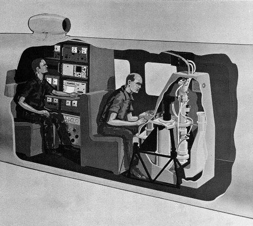
Figure 36 : An artist’s impression of the laser profiler/receiver (right) and electronics/services rack (left) in an aircraft.
The profiler/receiver is shown covered with a shroud that was to enable additional airconditioning of these units. The radiator is shown on the roof to provide heat exchange for the laser.
The basis of the measurement of the aircraft to ground distance was that the laser beam emerged from the bottom mirror of the laser with a diameter of approximately 3 millimetres. Passing through the modulator unit, the laser beam had its intensity modulated with a 3MHz sine wave. The modulated beam then passed through a diverging telescope which produced a 30 centimetre diameter spot on the ground at a distance from the terrain of 2000 metres. The receiving telescope, which had a field of view of about 60 centimetres diameter at 2000 metres, was aligned to the laser illuminated spot on the ground and received the reflected laser light from this area. The received signal was passed through a field stop and an adjustable interference filter of 4880 Angstrom, and on to the photomultiplier cathode. The output from the photomultiplier consisted of a small amount of the reflected 3MHz signal and random noise, the result of reflected sunlight. The equipment was designed with narrow bandwidths, both electrically and optically, to reduce this noise content. The received 3MHz signal was amplified by a head amplifier on the photomultiplier and fed into the signal channel of the profiler computer. A reference signal, which was a small sample of the transmitted signal was taken from the modulator driver and applied to the reference channel of the profiler computer. Both these signals were then amplified, limited, and compared in phase, the phase difference appearing as a direct current output suitable for recording.
The output from the laser terrain profiling system was recorded on two separate but correlated media. A photographic record of the actual profile against the terrain and a chart on which was recorded the continuous measurements. To accurately correlate the information on both media, a timing code was recorded on each. This record was located near each edge of the respective media to provide redundancy. Please refer to Figure 45 below. At the start of each flight the timing code generator was zeroed and each time the camera and/or chart recorder was run the timecode was recorded as long and short light flashes on each side of the film image and as equivalent square wave traces at the top and bottom of the chart. The timecode showed as short and long pulses each second, the pulse finishing at the commencement of the next second in all cases. To herald the minute, and thus indicate the direction of increasing time, long pulses (0.6 second duration) commenced during the 40th second of every minute, continued to the 56th second, followed by short pulses (0.2 second duration) for the 57th, 58th and 59th second. The 60th second was always a full one second pulse and thus it merged with the 59th second pulse to show as an extra long pulse (1.2 second duration). The 1st and 2nd seconds of the next minute were always short pulses. This heraldic sequence lasting 30 seconds from the 40th second was the same for each minute, so to distinguish one minute from the next a further use was made of long pulses. Commencing at the 10th, 20th and 30th seconds and counting the number of long pulses starting at 10th, 20th and 30th second marks, gave respectively the units of hours, tens of minutes and units of minutes since the time code generator was zeroed at the commencement of the flight. As the laser profiler and the camera were recording simultaneously it was possible to relate a point of detail on the photography to the chart values at that instant via the timecode and vice versa.
The photographic record was a strip of film up to 30 metres long and 70mm wide. The white line down the centre of the film strip was the path of the laser beam across the terrain. The chart was a roll of Ultra Violet (UV) sensitive paper about six inches wide and up to 50 meters long. In the final configuration a UV light source was reflected using galvanometer controlled mirrors to simultaneously place 7 traces of information on the chart, along with a 2mm grid with every fifth (one centimetre) line delineated for easier interpretation. The bottom centimetre line of this grid was used as a measuring reference as the chart paper was allowed to float in the cross direction as it was drawn past the recording optics. Please refer to Figure 45 below. The seven traces consisted of two for the timecode (top and bottom), the grid, terrain profile, Barometric Reference Unit, Statoscope, and gyroscope. The full technical specification is at Annexure F.
Sometime in 1969, the laser profiler project was given to John E Clegg, Optics and Surveillance Division, with Michael F Penny, Principal Officer, Laser Group, as the project team coordinator. Lines (1992) stated that it was Clegg and Penny who were largely responsible for integrating the varied range of instrumentation from laboratory design and testing through to a well designed operational field system which satisfied all the early concepts. The experimental system was installed, in 1969, in a Dakota DC3 flown and maintained by the Royal Australian Air Force’s, Aircraft Research and Development Unit (ARDU). After test profiles were acquired around Adelaide in February 1970, Lake Eyre was used as a profiling target and later in March 1970, the profiling system was taken to Canberra for demonstration.
As well as checking that the laser profiler operated satisfactorily in an airborne environment, profiles were acquired over different terrain and surfaces. These tests were necessary to ensure that the reflected laser radiation from the differing terrain provided a sufficiently strong return signal. For example, it was found that vegetated surfaces provided a stronger return signal than that from bare paddocks or desert. As the majority of Nat Map’s profiling would be of desert regions an adequate signal from such terrain was vital.
Profiles were thus obtained over urban/industrial, desert, salt lake, wooded terrain, grass and water targets. Figure 37 shows one of the earliest profiles over Parafield airport near Adelaide and demonstrated the sensitivity of the laser system in clearly defining the sawtooth profile of the hangar roof.
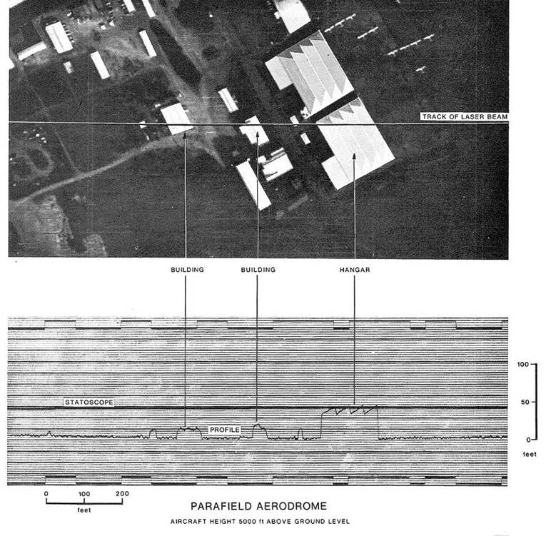
Figure 37 : One of the earliest Dakota trial laser profiles over Parafield airport near Adelaide.
The sensitivity of the laser system was sufficient to clearly define the sawtooth profile of the hangar roof.
Over the South Australian Gulf, satisfactory profiles of the water surface were obtained and even showed penetration to the sea floor. Lake Burley Griffin in Canberra was profiled on a number of occasions and yielded good surface profiles likely due to the Lake’s water being muddy after recent rains.
The Lake Eyre trials were more rigorous. A series of profiling runs were carried out along a surveyed track across Madigans Gulf at Lake Eyre (north). Since the lake’s surface height was already known, heights derived from these profiles showed operational system accuracy. Subsequent analysis of the Lake Eyre profiles confirmed that the laser transmitter-receiver performance exceeded the performance requirement which was that the root mean square height error shall not exceed 0.5 metres at an operational height of 2,000 metres above sun illuminated terrain which exhibits low diffuse reflectivity (i.e. desert).
While testing and trials of the laser terrain profiler had been carried out from a Dakota test aircraft final rack design and cabling was all dependant on Nat Map’s choice of aircraft. It would seem that Nat Map’s positive experience with the twin engine, high wing, Rockwell 680FL Grand Commander carrying the Aerodist system led it to tender for the same aircraft type to carry the laser profiler. A contract was soon let to Executive Air Services based at Essendon Airport, for VH-EXP (please refer to Figures 38 and 39 below). Executive Air Services, VH-EXZ was already contracted to Nat Map for Aerodist operations. Because of developmental requirements the initial contract for VH-EXP was for three years rather than the normal two year maximum for such contracts.
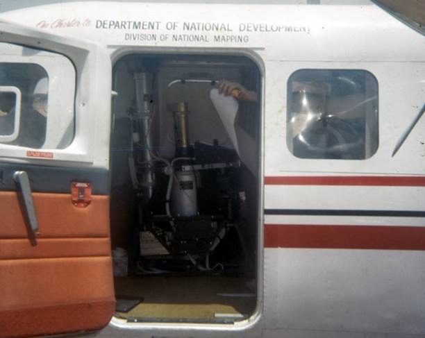
Figure 38 : Contracted Executive Air Services, Rockwell 680FL Grand Commander VH-EXP, showing exterior signage over cabin door.
With the selection of the Rockwell 680FL Grand Commander, WRE built a full scale wooden replica of the cabin section to ensure all equipment would fit when the time came. Included was a small radiator to be mounted on the top fuselage for equipment cooling. Installation of the laser profiler in the replica cabin, revealed that the laser receiver blocked the emergency access. With no way of modifying or repositioning the profiler assembly, an emergency device was purchased and a mount made to hold it safely. The device was a small axe which could be used to forcibly remove the obstructing equipment and permit access to the emergency window. Thankfully it never had to be employed, but many a new member of the crew was chilled by stories of its fictitious use before being told of its intended purpose. While WRE were resolving installation issues, Executive Air Services were modifying VH-EXP to supply the electrical power, hold the equipment and have holes cut in the floor and fuselage to allow operational use of the profiler. A list of the required modifications formed part of the aircraft tender documents and the list of required modifications is at Annexure G. The full configuration can be seen in Figures 40 and 41.
Nat Map’s Laser Terrain Profiler was installed in VH-EXP in May 1970. Initial flights with the equipment however, revealed a problem with the profiler mount. Not generally noticeable was that at cruise, the Grand Commander flew with a 4° nose high attitude. The profiler mount did not allow for such a large extent of adjustment to point the laser vertically. WRE quickly manufactured special shims and bolts which, when the aircraft was at cruise, had the profiler assembly at a near level orientation and allowed for the verticality of the laser to be adjusted as designed. Formal acceptance of the system occurred in July 1970, and subsequently, Nat Map flew its first laser profile in late 1970 outside Broken Hill.
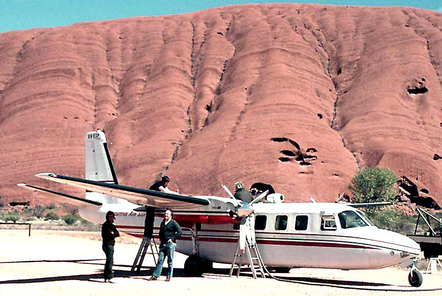
Figure 39 : Contracted Executive Air Services, Rockwell 680FL Grand Commander, VH-EXP on laser terrain profiling operations in 1975.
VH-EXP is being refuelled at the old Connellan airstrip at Ayers Rock now Uluru.
Under wing left is Ross Chisholm and right Paul Wise with pilot Phil Robertson on ladder at rear (Courtesy Ozcan Ertok).
One proposed aspect of the system design was never implemented; that of having the height above terrain output directly in metres, and the value imaged on the same roll of film as the terrain image from the strip camera. The most likely reason for this feature not being implemented was the Assistant Director’s, Joe Lines, concern of trusting technology too much. Joe did not want an expensive field operation to collect a mass of data only to find some time later that there were problems and some or all of these data were worthless. That would mean recollecting the data again. Joe wanted a process that could be monitored in real time, or close to it, and any problems overcome whilst on site. The Aerodist line crossing distances being recorded on a chart, monitored by an operator is an example. To this end the profiling system data were also output on a paper chart which the electronics technician was able to view at all times. The strip photography obviously could not be viewed in real time but small lengths of each film were exposed and simply developed in the field to ensure that the camera had been likely operating correctly. It was seen as impractical to try to develop 30 meter lengths of film in the field but regular shipments of the film and profiling materials back to the office where the films were professionally processed and assessed was found to be an adequate control of the photographic quality. Similar reasoning was given by WRE when asked why the profiler data was not stored digitally on then magnetic tape. The visual record would still have been required so the tape unit etc would have just been an added complication and expense!
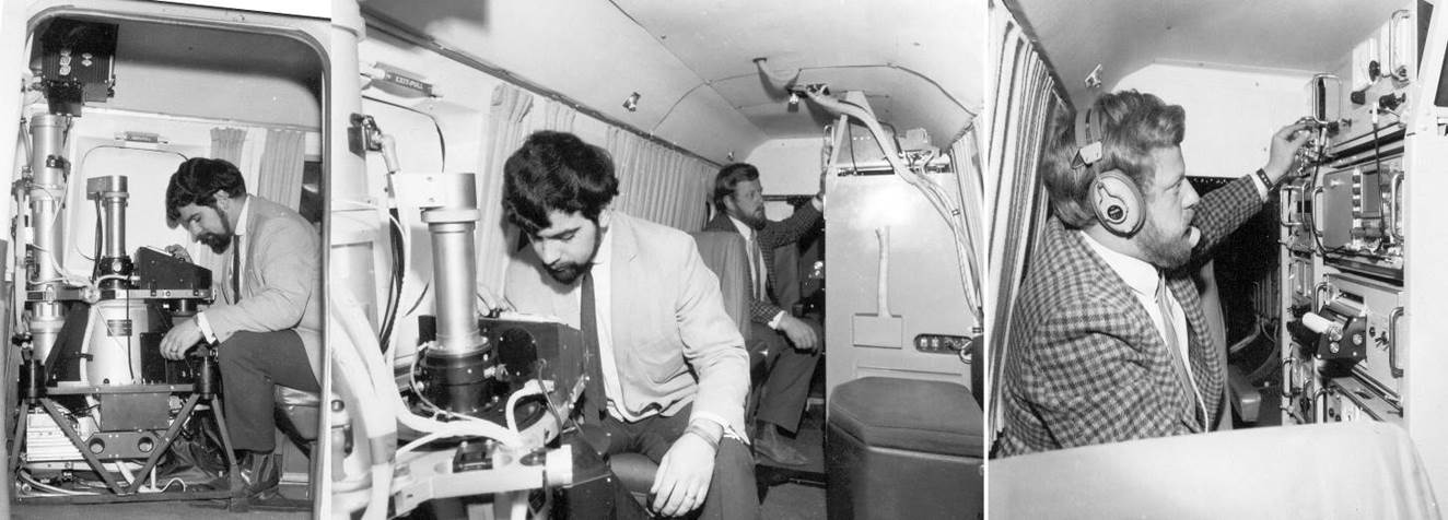
Figure 40 : Series of 1970 publicity photographs taken of the laser terrain profiler after installation in VH-EXP.
Left is the laser profiler assembly with Norm Edwards and right is the electronic equipment and services rack with Adrian Wright, centre shows layout of equipment in aircraft cabin. These photographs were taken before the installation of the B3 drift sight.
In 1973, WRE proposed that Nat Map utilise the newly developed sealed lasers. Sealed lasers were developed for the Army’s WREMAPS 11 system and as the name implies did not require a continuous gas supply to be provided to the laser tube. A major advantage of the sealed laser was seen to be that their operational life would have lasted for a complete field season, mitigating down time for laser changes. Although this development eliminated the gas supply equipment and some plumbing, Nat Map found that these lasers lacked the power of the original design. The terrain profiles became noisy at higher altitudes which in turn limited the amount of flying per day. For good profiling, smooth flying conditions were required. As turbulence developed during the day smooth conditions could only be found by flying at higher altitudes. If such altitudes could not be used, then profiling operations had to be curtailed. In the desert areas this limitation could not be accepted and so after a couple of months the decision was made to return to the original specification.
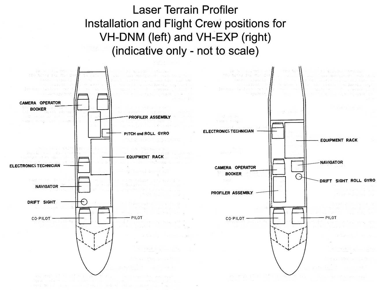
Figure 41 : Diagram showing respective operational configurations.
|
|
|
|
Figure 42 : Left photograph shows the profiler system installation in the NOMAD and the right photograph the NOMAD’s central hatch in the open position. |
|
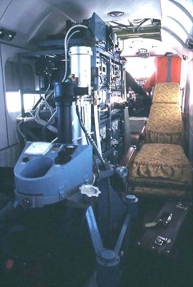
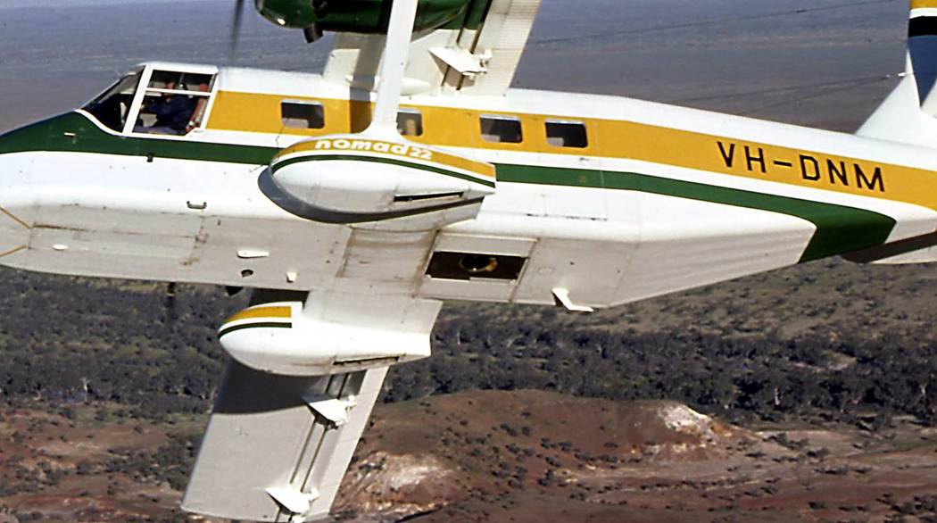
National Mapping purchased its own aircraft for aerial photography and laser terrain profiling in 1976. The Nomad N22B-25 aircraft (VH-DNM), manufactured by the then Government Aircraft Factory at Fishermans Bend, Melbourne, was powered by twin Allison 250-B17 series turboprop engines. From 1977 to 1979 the Nomad was the airborne platform for the laser terrain profiler.
The installation of the laser profiler system in the NOMAD only required a change to the positioning of the major assemblies specifically dictated by the NOMAD’s central hatch over which the profiler assembly had to be installed. The heavier electronic equipment and services rack was then installed close to the aircraft’s centre of gravity. The NOMAD layout can be seen in Figures 41 and 42 above.
In 1977, the laser profiling system was installed in the NOMAD for the first time at WRE. All went well and after ground testing only a test flight remained. After takeoff, aircraft electrical power was supplied to the laser system and slowly and carefully all the modules were tested. Again, no problems were encountered until all traces were viewed on the chart; the terrain profile was noisy and the laser output power could not be increased to reduce the noise. After landing and a conference of all concerned the problem was traced to the NOMAD’s battery. Simplistically while rated at a specific voltage, in this case 28 volts, batteries can sustain a slightly higher voltage. These one or two extra battery volts allowed the laser to generate extra power. Within a few days a suitable battery was acquired and installed in the NOMAD and the profiling system operated nominally for the next few years.
System Components comprising the Laser Terrain Profiler (LTP)
The Mark 1 laser profiling system consisted of two major assemblies: the profiler assembly, holding the laser tube, receiving telescope and a 70 mm tracking camera, and the electronic equipment and services rack, specially designed for the aircraft and holding a number of electronic modules, to control and monitor the profiler system and record the terrain profiler output. To complete the operational configuration a Wild RST2 Registering Statoscope measured the aircraft’s deviation from the isobaric surface during profiling; a Bendix Model B3, gyro stabilised driftsight, aided line navigation; and a Nikon F, 35mm frame camera, with motorised back and remote operation could record terrain events. The following is only a summary of the laser profiling system as details are already contained in Paul Wise’s, 1979 National Mapping Technical Report 26, Laser Terrain Profiler, available via this {a href=”report_tdnm/laser26/laser.htm”}link{/a}.
|
Laser Terrain Profiling Installation |
|
|
Profiler Assembly |
The profiler assembly, shown in Figure 43, held the laser tube, receiving telescope and slit camera in the same vertical alignment and was adjustable so that the three components all viewed the same area of the terrain. |
|
|
|
|
Figure 43 : The profiler assembly with laser tube, receiving telescope and slit camera. |
|
|
Laser transmitter |
A continuous wave, argon ion laser with a light output in the blue-green (0.488 micrometres) region of the Electromagnetic Spectrum. The laser tube, as shown in Figure 44 below, was water cooled, with the laser cavity supplied with a controlled flow of argon gas from a small storage cylinder and a vacuum pump controlling the flow of gas. The laser beam was intensity modulated (turned on and off at a high frequency) to finally emerge with a small divergence such that from an altitude of 3,000 metres it only illuminated an area of the terrain of less than 0.5 metres diameter. The intensity modulation permitted a phase comparison to be made between the transmitted and received signals giving a measure of the terrain height. |
|
|
|
|
Figure 44 : A laser tube with its transportation box. |
|
|
Receiving telescope |
A Cassegrain telescope, with an effective aperture of 0.18 metres and a focal length of 2.5 metres. The angular field of the telescope was limited by a field stop positioned in the focal plane that was 1.5 times the diameter of the laser beam diameter. This narrow field of view reduced as far as practicable the sunlight induced background radiation entering the receiver. A photomultiplier detected the return signal and controlled the sensitivity of this system. The receiver axis was fixed with respect to the profiler structure and alignment of the whole system was affected by tilting the laser transmitter. This facility had been arranged by mounting the laser and modulator on a ball joint with the centre of rotation near the focus of the expanding telescope input lens. In practice by monitoring received signal strength the electronics technician could readily tilt the laser in flight to optimise alignment. |
|
Strip camera |
A cassette loading 70mm strip camera provided photographic evidence of the track of the laser spot on the ground at a data rate of 25 points per second. The camera incorporated a 7 inch (177.8 millimetres) focal length Kodak Aero Ektar Lens with a fixed aperture of f 2.5. A window set at 45° to the lens axis reflected the incoming rays to the film set at the focal plane just beyond a narrow slit. Nominal photoscale was 1: 15,000 at 2,000 metres above terrain. In 1973 an 88.9mm focal length lens was fitted to give a nominal photoscale of 1: 25,000 as shown in Figure 45 below. The change of camera lens was to facilitate transfer of selected points on the laser profile to the mapping photography. Since the window was partially transparent the ground was also imaged on a screen which was viewed by the operator through a rotating disc engraved with a spiral. The speed of the disc was adjusted such that the ground image of the terrain below and the spiral appeared to be moving at the same rate across the operator’s field of view. As the disc (please refer to Figure 46 below) was driven by the film transport motor this adjustment to the disc speed ensured equal longitudinal and transverse film scales. Additionally, the camera could be rotated to compensate for any drift of the aircraft. The amount of rotation required was set by aligning the ground image motion with straight lines engraved on the viewing screen and ensured that the slit was always normal to the ground track and produced an undistorted picture. Automatic aperture control was achieved by a servo controlled neutral density wedge positioned in the front of the slit. The wedge maintained a constant film exposure under varying ambient light conditions. Six magazines capable of holding rolls of 70mm film, generally Kodak Aerographic 2402, up to 30 metres in length were supplied. |
|
|
|
|
Figure 45 : Section of 70mm Slit Camera photography. |
|
|
|
|
|
Figure 46 : Operator’s panel on the profiler assembly to control the 70mm strip camera showing (lower centre) the engraved rotating disc spiral and its speed control knob right; strip camera automatic exposure gauge and frame counter for 35mm frame camera are top right. |
|
|
Electronic equipment & services rack |
The rack shown in Figure 47 was designed to fit the aircraft cabin and hold, shock mounted, electronic modules, to control and monitor the profiler system and record the profiler output. |
|
|
|
|
Figure 47 : Electronic equipment and services rack with its modules. |
|
|
Profiler computer |
The distance to the terrain below the aircraft came from measuring the phase difference between the transmitted laser signal and the return signal. The profiler used a modulation frequency of 3MHz so that each wavelength corresponded to a height change of 50 metres. Over steep terrain there may be too many 50 metre steps to interpret correctly. Thus in 1971, a coarse mode (0.5Hz), where one phase change equalled 300 metres variation in terrain clearance, was introduced and could be switched in briefly (1-2 seconds) when required. To indicate that the mode had been switched the Mode Trace on the chart, usually a straight line, would deviate down while the coarse mode was being used. During this time the laser trace would briefly change in apparent noise level and a change in trace position. |
|
Timing unit |
To correlate the laser profile with the photographic record of the terrain, coded pulses (timing code or TIMCODE, please refer Annexure H) were recorded simultaneously on both media. The pulses represented seconds of elapsed time, generally from system start, and were displayed on the front panel of the unit like a digital clock, for the electronics technician’s information. The pulses on the chart and film were in a coded format which allowed any instant to be converted to hours, minutes and seconds. The timing code is illustrated in Figure 48 below, and shows how the code was translated into hours, minutes and seconds of elapsed time. |
|
|
|
|
Figure 48 : The timing code pulses and their translation into hours, minutes and seconds of elapsed time. |
|
|
UV recorder
|
The chart recorder was an adapted 12 channel SE Laboratories Ultraviolet (UV) recorder type SE3006. The unit had been extensively modified to operate from 28 volts and a self spooling device had been added. A mercury vapour tube produced ultraviolet radiation which was reflected onto sensitive paper by mirrors controlled by the electrical outputs from the various instruments and also generated a background graticule. Potentiometers could vary the intensity of the traces and graticule. UV sensitive, Kodak Linagraph Direct Print Paper, Type 1895, which came in rolls 6 inches wide and 150 feet (50 metres) long, was used to contain the permanent record as shown in Figure 49 below. |
|
|
|
|
Figure 49 : Section of UV chart showing traces from the various instruments and relationship to features in the terrain as captured by the 70mm Slit Camera. |
|
|
Converter and regulator modules |
The aircraft’s 28 volt supply was converted to power the laser. |
|
Vacuum and Water modules |
The Vacuum Unit supplied a controlled flow of argon gas into the laser cavity whilst maintaining an absolute gas pressure of approximately 100 microns. The water cooling unit pumped water through the laser to absorb the heat generated by the laser arc discharge, the magnetic field and the directly heated cathode. The water was cooled in a fuselage mounted heat exchanger. |
|
Oscilloscope |
Type 422 for monitoring and general testing. |
|
Additional equipment |
|
|
Pitch and Roll Gyroscope (also known as the VRG or Vertical Roll Gyro)
|
The amount of aircraft movement from straight and level flight was indicated on the chart via the pitch and roll gyroscopes. The variation in the gyroscope’s traces indicated regions where the aircraft’s movement meant that the laser was not vertical and the height obtained was false. The two directional gyroscope was introduced in 1974. Prior to this lateral roll of the aircraft was measured by a pick-off modification of the gyroscope in the Bendix B3 drift sight introduced in 1971. |
|
Frame camera |
A wide angle, 35mm, Nikon F frame camera, with a motorized back was incorporated into the system. Mounted under the aircraft cabin floor to focus on the terrain below, it was operated by remote control. While 30 metre rolls of 35mm film could be loaded into the camera, in practice readily available 36 frame, 35mm film was used. |
|
Recording Statoscope |
A Wild Statoscope type RST2 was used for about five years to measure the deviation of the aircraft from a constant pressure surface selected at the start of each profiling line. This equipment comprised a sensitive differential pressure transducer and a stable pressure reference source. Prior to the start of a profiling line both inputs to the pressure transducer were connected to a balanced arrangement of static pressure vents located on each side of the rear fuselage. At the start of a line the reference cavity of the transducer was then sealed off and the reference pressure held constant for the duration of the line by maintaining the cavity at a constant temperature. While operationally reliable the RST 2 drew excessive electrical power and was overly heavy. This equipment also required some 2 hours for the oven temperature to stabilize before use. It was replaced by the WRE, designed and manufactured, Barometric Reference Unit (BRU). The Statoscope and BRU were operated in parallel for several years to ensure that the BRU was completely reliable and the Statoscope could be made redundant. |
|
Barometric Reference Unit (BRU) |
After being operated in parallel with the abovementioned Statoscope from 1971 and found to be completely reliable and accurate, the BRU replaced the Statoscope for the remainder of the laser terrain profiling program. |
|
Bendix B3 Drift Meter or Driftsight (as shown in Figure 50 below) |
Not part of the original installation but installed in 1971 for improved line navigation and measuring aircraft drift. This gyroscopically stabilised, optical instrument protruded through the lower fuselage and could be rotated through 360 degrees. A prism, controlled by the operator, allowed the operator to view the terrain in an arc from the horizon to vertically below the aircraft. |
|
|
|
|
Figure 50 : Bendix B3 gyroscopically stabilised driftsight being operated by Peter Quinn. |
|
|
Automatic Pilot
|
Introduced in 1971, a three axis autopilot unit with height holding capability was utilised to ensure the aircraft was maintained within a 50 metre vertical envelope at all times during profiling. While it was possible, it was considered not practical, to fly the aircraft manually within this ±25 metre criteria throughout the usual 4 to 5 hour operational flight. The Bendix M4C or Collins AP107 were used at different times. |
|
Support Vehicle |
Nat Map’s experience with its Aerodist party having a transportable electronics workshop/office saw WRE modify a 4 ton Bedford RLCH 4x4 chassis for a similar role with the laser terrain profiling system. Of note was the darkroom, purpose designed testing panels, electrically driven chart handling roller, and map storage draws. For testing the laser profiler equipment on the ground, a power supply unit was mounted externally. The concern was that if any part of the ground unit failed the consequences might have been catastrophic for the profiler. Thus, it was rarely used and finally not taken into the field after 1975. If testing of the profiler equipment could not be done safely in the air it was preferable to return to WRE where their ground power unit was highly reliable. In 1976 the electronics workshop/office was transferred to an International C1600 series four wheel drive chassis. The vehicles were both known as the laser caravan. Please refer to Figures 51 to 55. |
|
|
|
|
Figure 51 : Modified 4 ton Bedford RLCH 4x4 laser caravan from passenger’s side. |
|
|
|
|
|
Figure 52 : Modified 4 ton Bedford RLCH 4x4 laser caravan from driver’s side. |
|
|
|
|
|
Figure 53 : Laser caravan interior - office area (left photograph) and electronics workbench (right photograph), with darkroom at left in the right photograph. |
|
|
|
|
|
Figure 54 : International C1600 series four wheel drive with laser caravan. |
|
|
|
|
|
|
|
|
|
|
|
Figure 55 : The above two photographs taken in 1971 at Mildura airport show a rare occasion where the ground power supply unit was used to power the laser profiling system and the laser beam’s reflection in the lower photograph (courtesy Laurie Edebohls). |
|
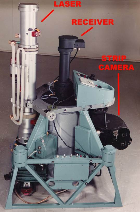
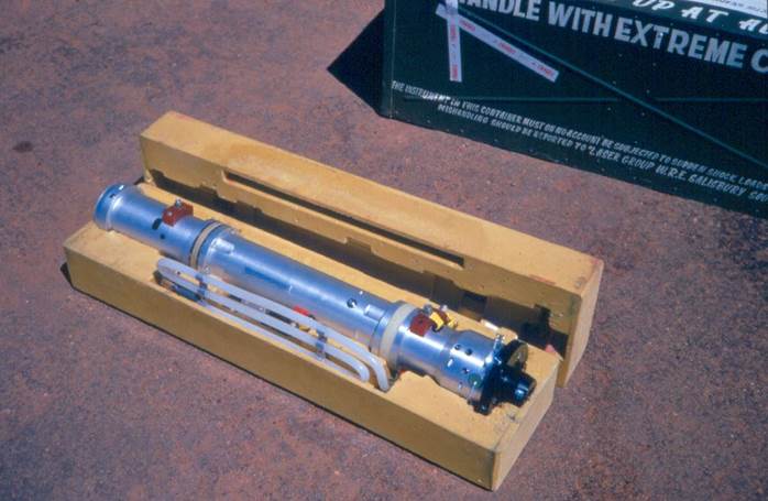
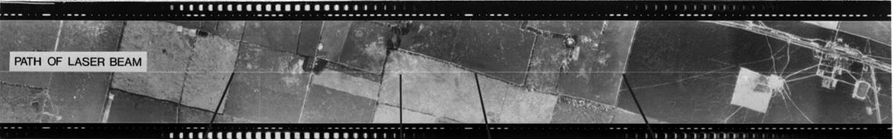
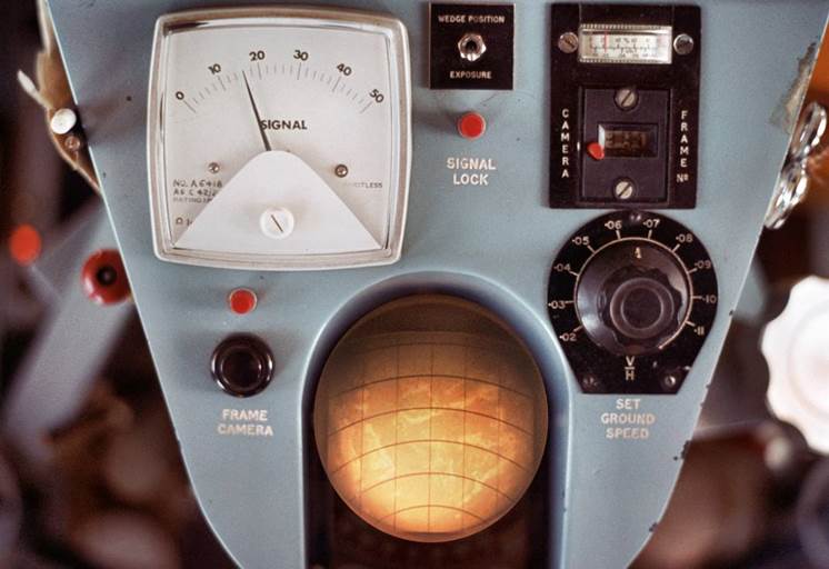
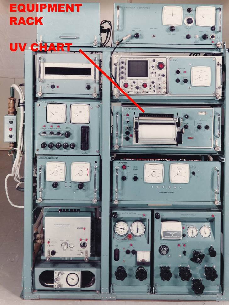
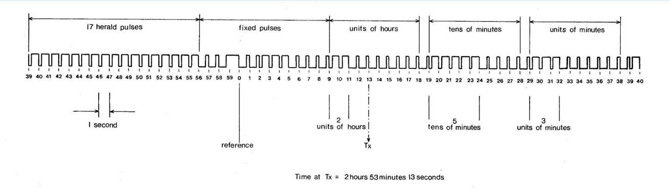
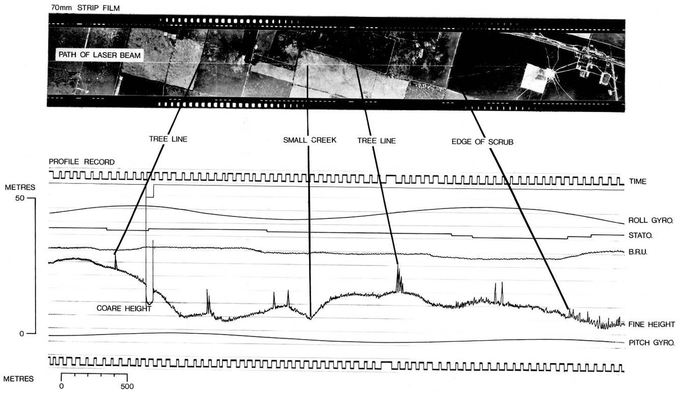
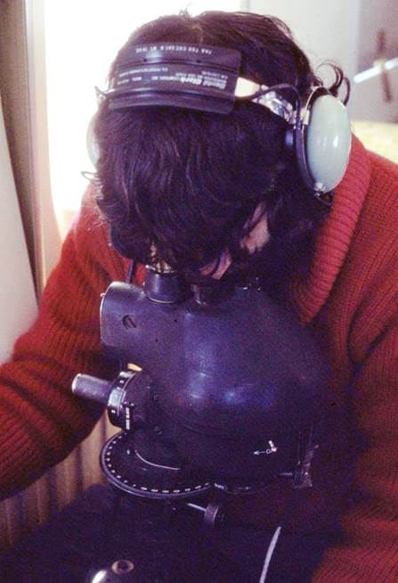
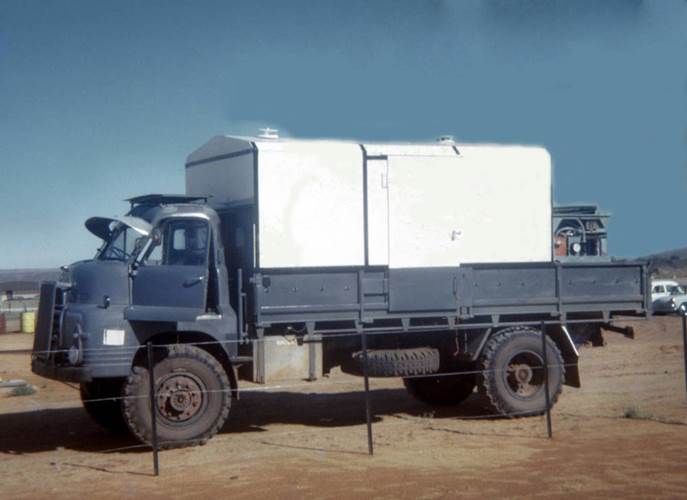
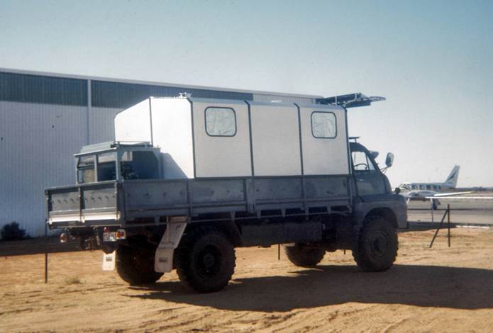
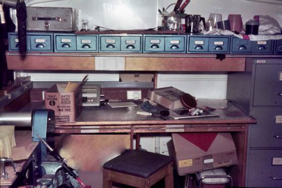
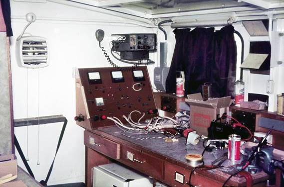
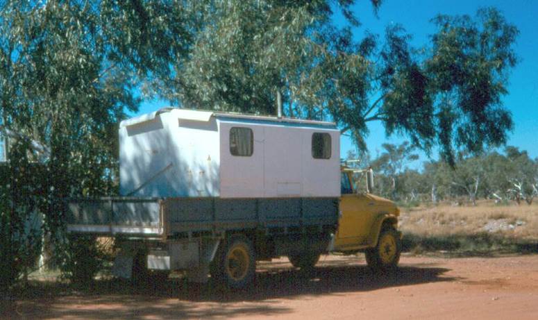
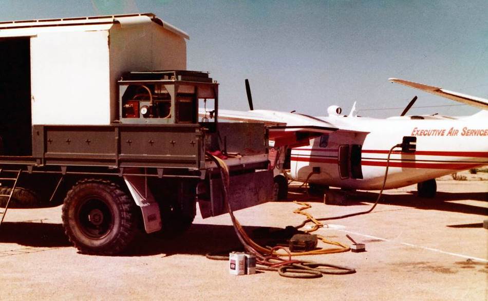
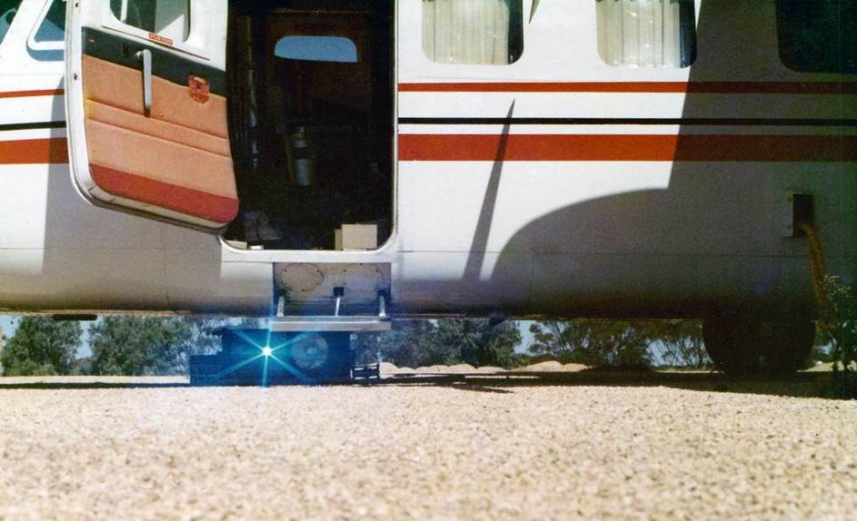
The expected life of the laser was in excess of 100 hours and when a laser became unserviceable it was returned to WRE for refurbishing. Four lasers were manufactured for Nat Map. It was anticipated that a spare laser tube would be transported in a specially designed case by the laser caravan. However, there was concern that despite this protection, given the poor roads the caravan would have to transit, the spare laser tube may prove to be unserviceable when needed. The most efficient solution was for the laser tube and its transport case to be held at WRE. On the failure of a laser in the field, WRE immediately airfreighted a replacement laser tube to the destination requested by Nat Map. This destination was usually the nearest major town with a daily airfreight schedule. If the profiling field party was not based there already, they would fly there to collect the shipment. A laser changeover was fairly simple. The removal of some connectors and the lifting out of the relatively light weight faulty laser tube, then reversing the process. The faulty laser was put into the transport case and returned to WRE. The new laser was then tested and if satisfactory normal operations recommenced.
During the 1970s Dr Michael F (Mike) Penny was Principal Officer of the Laser Group at WRE. The main members of Penny’s team included :
|
Alf Gos Gosling |
WRE’s liaison officer for Nat Map – Gos facilitated the solving of any problem that arose with Nat Map’s laser profiler and brought in those below as necessary |
|
Ralph Abbot |
Electronics systems |
|
Don Rees |
Laser system and refurbishment |
|
Brian Woodcock |
Mechanical systems |
|
Penny, Gosling and Woodcock photographed in Figure 56 below. |
|
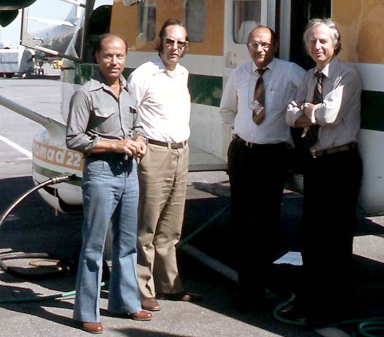
Figure 56 : Photograph at WRE with Nat Map’s Nomad aircraft (L-R) Nat Map’s Ozcan Ertok with WRE’s Brian Woodcock, Alan Gosling and Mike Penny (courtesy Ozcan Ertok).
Those Natmappers who had the pleasure to work with any of the above appreciated their expertise and enthusiasm with which they assisted Nat Map. The role of these WRE personnel was significant in the overall success of the laser terrain profiling program.
Laser Profiling Field Support Vehicles
As mentioned above the laser field party used two chassis for its caravan; a Bedford, replaced in 1976 by an International. The Bedford RL series were manufactured in England from the early 1950s to the late 1960s by Vauxhall Motors Limited a division of the General Motors Corporation. The RLCH models of these cab-over-engine trucks were operated by National Mapping between 1960 and 1974. (The RLCH stood for R series, long wheelbase version, cab-chassis configuration, heavy duty.) This model had a carrying capacity of over 4 tons (about 4 tons 10 hundredweight tare and 8 tons 14 hundredweight gross vehicle weight). The engine was a 4.9 litres (300 cubic inches) capacity 6 cylinder overhead valve petrol engine that developed 110 brake horse power (82 kilowatts). Transmission was via a 4 speed gearbox and a 2 speed transfer case that gave a 2:1 reduction in low range. Four wheel drive was only available in low range. The brakes were assisted by a Clayton-Dewandre vacuum servo system. Tyres of the size 11.00 x 20 were fitted to Nat Map Bedfords. The wheels on these vehicles had removable side bands (split rims). Most of Nat Map’s Bedfords had a small air compressor for inflating tyres. The compressor was driven by a power takeoff from the vehicle gearbox.
The International C1600 was fitted with a 6-281 International petrol engine of 282 cubic inches (4.6 litres) displacement. The engine produced 142 brake horse power (106 kilowatts) at 3,800rpm and 241 foot-pounds (327 Newton-metres) of torque at 1,800 rpm. The transmission in these vehicles was by a 4 speed gearbox with a 2 speed (high and low range) transfer case. Size 10.00 x 20 tyres with 12 ply rating were fitted to the C1600 International. The wheels on these vehicles had removable side bands (split-rims).
Transport for the aircraft crew and general support duties was initially by a 6 cylinder 4 wheel drive Toyota Land Cruiser FJ55 series station wagon, as shown in Figure 57 below. The petrol engine had a capacity of 3.9 litres. It produced 112 kilowatts of power (150 horsepower) at 4,000 rpm and 290 Newton-metres (214 foot-pounds) of torque at 3,000 rpm. This vehicle had a 3 speed manual transmission with a 2 speed (high and low range) transfer case. It was fitted with 7.60 x 15 tyres on wheels that had removable side bands (split-rims).
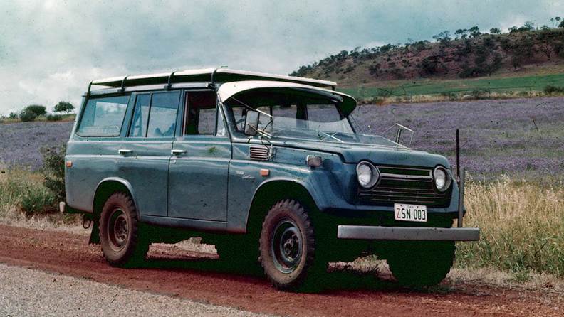
Figure 57 : Laser profiling party ground transport Toyota Land Cruiser FJ55 series station wagon, ZSN003 (courtesy Laurie Edebohls).
After the Toyota was severely damaged on a Nullarbor track, transport became a Land Rover Series IIA, 109 inch wheel base utility with integrated metal canopy. These vehicles were powered by 2.25 litre capacity 4 cylinder petrol engines that had an overhead valve configuration. These engines produced 55 kilowatts of power at 4,200 rpm and 160 Newton-metres of torque at 2,000 rpm. The transmission was by a 4 speed gearbox with a 2 speed (high and low range) transfer case. These vehicles were fitted with 7.50 x 16 tyres on well-based rims. In 1973 a new Toyota became available and this vehicle was used until the end of 1975.
The desert operations of 1976 saw fuel and support equipment transported to Kidson Field using International C1600 and C1300 series vehicles. The C1600 was the same chassis as described above except it carried a canvas covered tray. The C1300 chassis was fitted with a 6-281 International petrol engine of 282 cubic inches (4.6 litres) displacement. The engine produced 142 brake horse power (106 kilowatts) at 3,800rpm and 241 foot-pounds (327 Newton-metres) of torque at 1,800 rpm. The transmission in these vehicles was by a 4 speed gearbox with a 2 speed (high and low range) transfer case. Size 8.25 x 16 tyres with 10 ply rating were fitted to C1300 Internationals. The wheels on these vehicles had removable side bands (split-rims). These vehicles were made in Australia by the International Harvester Company at its assembly plant in Dandenong, Victoria.
The International C1300 had a metal cabin and metal utility style bodies with canvas canopies. These vehicles had a manufacturer’s gross vehicle weight rating of 8,700 pounds and a tare weight of around 5,200 pounds. Thus, they had a payload of about 3,500 pounds (1,500 kilograms). The standard Nat Map fit out provided two 14 gallon capacity fuel tanks (one under each cabin door), a 60 gallon capacity auxiliary fuel tank and a 40 gallon capacity water tank. Nat Map vehicles all had manual transmissions and were devoid of present day comforts such as air conditioning and power steering.
During 1976 it was seen to be advantageous for aircraft crew transport to be provided by hire car. The Commonwealth Government’s contracts with commercial hire car companies were seen to offer more cost effective vehicle transport in most major towns. Until the end of the laser flying program unless operations called for specialised Nat Map vehicle support, hire cars were used. Of necessity the laser caravan was still driven from base to base.
Laser Terrain Profiling Operations in Nat Map
Preparation
Laser terrain profiles were acquired over specific blocks of 1: 250,000 scale map sheets, as described above for APR. An example of the positioning of LTP flight lines along the lateral overlap of successive strips of aerial photography is shown in Figure 58 below. The significant difference with the LTP flight line configuration was that the north-south flight tie lines were altered slightly to pass over any convenient bench marks that could then be used as height datum points.
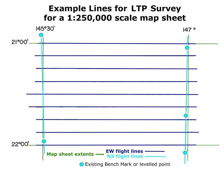
Figure 58 : Example of the LTP flight lines required for a standard 1: 250,000 scale map sheet of 8 strips of aerial photography.
Initially however, laser profiling operations in the field mimicked radar profiling operations. Datum airstrips were overflown at the start and end of each flight to enable the Henry correction to be determined for the laser profiles. It was soon realised that with the smaller and more accurate laser footprint extensive flat areas were no longer needed for datums. Bench marks along roads or tracks could now be used as long as the surrounding terrain was flat. Points on hills or slopes were avoided however, so as not to introduce any error in projecting the height from the bench mark to the laser profile.
The adoption in 1971 of bench marks as profile control favourably impacted flying operations. The previous requirement to climb to altitude after takeoff and fly a datum run as well as the same prelanding datum run requirement was removed. After takeoff the aircraft could now head for the operational area while climbing to altitude and the profiling system was made ready. More flight time was thus available in the operational area. The most frustrating operational aspect was also removed in that a whole flight’s profiling could be wasted if for any reason the prelanding datum run was not achieved. As shown diagrammatically in Figure 54, a laser profile was considered acquired provided it crossed a bench mark at the start and finish of any north-south tie line or for east-west lines they crossed a north-south tie line at the start and finish.
In the early years of laser profiling the use of bench marks brought the inherent problem of inconsistent height datums. Prior to the establishment of the AHD, a variety of state, rail and local vertical datums existed. Before any bench mark was adopted for use as profile control, its datum had to be established. Due to the lack of complete documentation being readily available this sometimes meant that an informed guess had to be made. In Queensland the Dajarra datum threw up problems time after time. This local datum was used extensively in western Queensland and was some 2 metres different from AHD. This datum difference was large enough that it could not be ignored but too small to be picked up in the laser profiling. Nevertheless, not all levelling in this region used this datum. As required, various Nat Map field parties were tasked with levelling to required bench mark traverses to enable a local AHD standard to be adopted. By the 1970s the AHD network as shown in Figure 59 had been adopted, and all bench marks now had an AHD height.
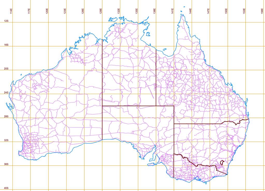
Figure 59 : Third order levelling traverses of the Australian Height Datum (AHD) at 1971.
As the laser profiles were to provide height data to control previously acquired aerial photography the required profile flight lines were drawn on a series of these photographs that had been taped together to form a long roll called a navroll (short for navigation roll). On one flight strip of photographs the extent of the side overlap from the flight strip above and below, was marked. These marks across the top and bottom of the strip were used to draw a centre line between the mark and photograph’s edge, indicating the centre of the side overlap area, and thus the required path of the planned profile once in the field. Generally, this procedure meant that only every second flight strip was required to be made into a navroll. Selected photographs were also made into navrolls for the north-south tie lines. In some areas these navrolls extended across up to four 1: 250,000 map sheet areas.
For administrative recording and identification, each planned profile line was given a unique 4 digit number and this was recorded on the navroll and any planning maps. As described in the section above the planned laser profile lines were also coded with the APR prefix and state alphabetic identifier (B-Queensland, C-New South Wales, D-Victoria, E-South Australia, F-Western Australia, G-Northern Territory). Any profile flown along a state border incorporated the state codes of both states. For example, a Western Australia laser profile line might be identified as APR/F/2345, a Victorian laser profile line as APR/D/1307 and a laser profile line along the Queensland-South Australia border as APR/BE/1789. This unique identification system later allowed any profile material to be registered, stored and retrieved on demand.
On each east-west navroll the position of the planned north-south profiles was marked and annotated. Likewise, on each north-south navroll the planned east-west profiles were annotated and marked. In the field this allowed the navigator to visually check each crossing and for the relative profile identifier and crossing time to be recorded in the flight log. This procedure saved time during office processing as all crossings could be identified immediately by their logged crossing time allowing them to be found more easily on the chart and film record.
Along with various maps covering the profiling area and to allow navigation to and from the airfields to be used as bases for the flying operations, the navrolls were packed and identified for transport.
It was found advantageous to provide a map of the profiling operations showing the line numbers in their approximate geographical position for the nearest then Department of Transport, Flight Service Unit (FSU). Leaving a copy of the map with the FSU after explaining the operation meant that official flight planning by the pilot was much easier. Line identifiers rather than tedious latitude/longitudes could be quoted and both the pilot and the FSU always knew the aircraft’s location.
Apart from the pilot, the laser profiling field party generally comprised a party leader who was also the flight line navigator and ensured precise tracking along the profile line (the pilot retained overall legal responsibility for safe aircraft navigation), an electronics technician and a strip camera operator/booker. A fifth logistics and support member usually stayed on the ground during flying operations undertaking various tasks to ensure the flight crew could maximise flying time. Other support and relief personnel or personnel undergoing training often increased the field party from five to eight members. In 1977, laser lines were profiled in areas of the Gibson and Great Sandy Deserts of Western Australia that were beyond the Nomad’s normal operational endurance. To overcome this operational constraint, the remote Kidson airstrip was used as a refuelling base during flights. Prior to the Nomad first landing at Kidson for this purpose, Laurie McLean and Tony Maginn trucked in supplies of aviation turbine kerosene and rehabilitated the surface of the airstrip. The rehabilitation was achieved by use of a drag scraper towed behind a D1310 International and by manual pick and spade work. This fuel support party was later relieved by Bob Goldsworthy and Roy Turner. The logistical support arrangement enabled some 1,000 kilometres of laser terrain profile to be captured daily in two flights of 500 kilometres each.
Laser Profiling Operations
A profile had to be acquired in a continuous direct line from start to finish. For a north-south tie line the start and finish were designated ground control points of known height, usually bench marks with an AHD height. An east-west profile had to start before a tie line and end after crossing another tie line. If there was equipment failure or the navigator got lost the line would be aborted and require reflying. Film magazine changes were avoided during profile acquisition as much as possible as the pictorial profile record lost could be extensive. Although a film jam might be noticed almost immediately and rectified, the risk of later finding that too much of the profile film record had been lost was not economical. It was considered more prudent to abort the profiling, replace the magazine, check that the replacement magazine was operational and refly the line. Chart changes took only a few seconds; also, the technician could see that the end of the chart was approaching and could coordinate with the navigator to ensure the change of chart would not occur at a critical time. Experience showed that if there was any doubt about the quality of the profile obtained it was better to refly a profile whilst in the area than to wait for it to be rejected back in the office. All sorts of other electronic failures happened from time to time requiring flying operations to be abandoned until the problem was solved and operational reliability was restored.
Navigation was carried out using a Bendix B3 gyrostabilised driftsight that protruded through the skin of the aircraft providing a 360 degree view of the terrain below. The B3 had a graticule along the fore/aft axis and a prism under the instrument that could be tilted to give a view anywhere from the forward horizon to just aft of the vertical. With a vertical view of the ground beneath, the graticule was rotated such that an object in the terrain tracked parallel to the graticule. The angle of rotation was read from the scale and noted as this was the angle of drift. Rotating the prism to give a view as far forward of the aircraft as possible to a feature on the planned profile path and correcting the aircraft’s heading to fly to that feature gave the required profile of the terrain. As each new feature was identified from the navroll and in the terrain, drift was checked and adjusted and heading corrections made until the extent of the profile was acquired. It was imperative that the aircraft be kept straight and level during profiling so any turns were kept small, in the order of a degree or so.
Profiling was carried out from an altitude of around 7,000 feet (2100 metres). This altitude was low enough to get a good return signal from the reflected laser beam and high enough to eliminate any turbulence for a few hours during the Australian winter months. All profiling was flown with the aircraft on autopilot. This ensured that the range of altitude in which the Statoscope and later BRU could operate was not exceeded. The autopilot was so crucial to good profiling that its failure meant the temporary suspension of flying operations. Profiling flights could last up to six hours on a good day but the norm was usually about five.
A typical flight started with the day’s crew arriving at the airstrip with the necessary navrolls, maps etc. Generally, a wide selection of navrolls was carried in the aircraft in case cloud or weather caused a change of plans in flight. In addition, the case containing the six fully loaded, 70mm film magazines was put aboard the aircraft along with any new supplies like boxes of Kodak UV recording chart, flight record sheets etc. The plan was to fly early and try to achieve the profiling before any turbulence started to interfere with aircraft stability. An early start also avoided mid-level cloud appearing during profiling. In at least one year as summer approached takeoff was planned for first light; by definition the time of first light is before sunrise. The alarm was thus set for 4AM and pretakeoff preparations were all done with the aid of a torch. The aircraft took off as soon as it was legal to do so and thus take advantage of the cool stable morning air for as long as possible.
After takeoff the pilot would switch on power to the laser terrain profiler system and the electronics technician would start to power up the profiler. Being able to isolate the laser profiler electronics from the aircraft’s electrical supply was a required safety feature. Should an aircraft problem arise, if required, the electrical load of the laser profiler could be shed immediately by the pilot and reduce the load on engines and generators. The 70mm camera operator/booker would install a film cassette and check camera and spiral operation. One important task for the camera operator/booker was to remove the protective slide. This slide prevented any material being thrown up during takeoff or landing and damaging the receiver and/or camera lens. When requested by the technician this person would also open the vacuum isolating taps on the laser. When not in operation these taps held the vacuum inside the laser and helped prolong the life of the laser’s internal components.
At the beginning of the laser system startup the technician would start the timecode generator. The coded pulses from this unit were simultaneously recorded on both the chart and film as the means of correlating the two media. The pulses represented seconds of elapsed time and were displayed on the front panel of the services rack like a digital clock, for the electronics technician’s information. Later a slave clock was introduced that could be more easily read by the booker. The starting of this unit was noted against standard time so events could be translated to actual time of day if required. For the most part however, this was never done and the chart and film time was just used as a convenient standard reference against which the electronics technician and camera operator/booker would log specific activities throughout the flight. A sample Survey Flight Record is shown at Figure 60 below. The technician separately would note voltages, amperages, pressures, flow, signal strength and overall time of laser operation. The laser profiler needed some 20 minutes to become stable and ready for operations thus the first line to be profiled was selected, if possible, to be at least that flying time from the base.
During the transit period, the navigator and pilot would consult and agree on a suitable feature in the terrain which the pilot would use to orient the aircraft on the run in for the first profile. In featureless or sandridge country it was found best to select the first profile line of the flight as the one which had a significant feature in the terrain which could be used as a navigation start point. Thus, profile lines were not necessarily flown in a rigid sequence but a sequence that met efficient use of flying hours.
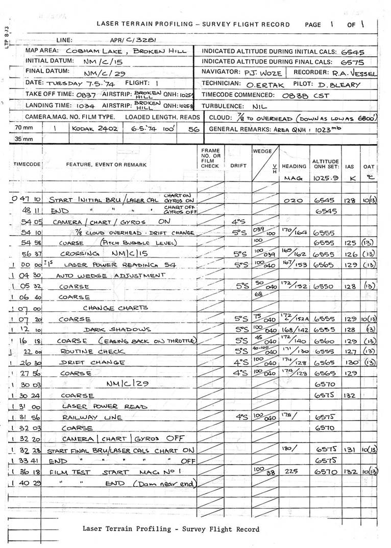
Figure 60 : Sample Survey Flight Record.
If the crew acknowledged their equipment was ready the aircraft would be headed down the line. As soon as the aircraft stabilized on a heading for the first profile line the navigator would take a drift reading and call for any heading correction. Next, the electronics technician was asked for Cals. Cals or Calibration sequence was a standard set of operations designed to make the main recording devices output their full extents onto the UV chart so that later the chart value could be converted to an actual value in meters.
Firstly, the laser profiler trace was made to trace its full extent of 100 millimetres across the chart. The extent was never precisely 100 millimetres but the extent was equal to 50 metres in aircraft to terrain distance, thus the actual ratio, distance change in metres per millimetre across the chart, could be calculated.
Next the Statoscope was calibrated but as this unit was later replaced by the Barometric Reference Unit (BRU) and the calibration technique was similar for the BRU only the BRU calibration is detailed here.
The Static Vent Valve on the BRU was checked to be open to the air outside the aircraft. The Reference Capsule Venting Valve was opened for about 3 seconds and then closed. The Calibrate Knob was depressed and held for about 3 seconds and then released. This procedure was repeated to provide 3 to 5 calibration pulses on the chart. After the last calibration pulse the Reference Capsule remained closed. This captured a sample of the air at that altitude against which any subsequent slight rise or fall of the aircraft from that altitude could be detected and measured. Again, these calibration pulses permitted the ratio of millimetres across the chart to the height change, in metres, of the aircraft to be calculated,
With the calibrations completed profiling could commence. At least a couple of minutes before the first crossing of another profile line or bench mark indicated on the navroll the navigator would ask for camera on, chart on. With the profiling system operating nominally the navigator would then call the crossing of the first item indicated on the navroll. The time of crossing as indicated on the system’s timecode display would be noted by the camera operator/booker. Along the line, drift, heading, outside air temperature, indicated air speed, chart changes and any other item indicated on the navroll, would be recorded by the camera operator/booker. The electronics technician would also be recording the system’s performance as an aid to forecasting and/or diagnosing any problems. After the last required item indicated on the navroll was crossed and both operators were satisfied that their equipment was still nominal another set of Cals were acquired. The navigator would then ask the pilot to turn towards the next planned profile line and the procedure would be repeated.
At the completion of profiling operations while returning to base the electronics technician would shut down the profiling system. The profiling charts would be collected and roughly annotated for further collation back at base. The 70mm camera operator/booker would mark and expose a short section of film for developing back at base as a check on camera operation. The operator would then pack away all used film cassettes ensuring they could be identified for later film removal and replenishment. When requested by the technician this person would now close the vacuum isolating taps on the laser helping to keep a high vacuum in the laser between flights. Lastly and again importantly, the camera operator/booker would replace the protective slide. After landing, all charts, the film cassette case and all recording sheets were removed from the aircraft and taken back to the field office.
Before the day’s work was considered complete exposed film was removed from the magazines and new film loaded. The section of film exposed to confirm camera operation was removed, developed and inspected. If this section of the film indicated no camera related problems then all that days’ films were deemed acceptable. The charts would be wound onto wooden rollers to facilitate handling and later processing. During this procedure the traces were visually inspected for clarity. If a chart change had occurred then the two sections of chart were taped together. If a chart contained more than one line of profile the chart was cut to separate the discrete profiles. Each end of the discrete profile charts was then stamped and annotated with its number, date acquired, and extent. When and if time permitted initial work could be started determining each chart’s calibration details. More on this aspect is described later. When a sufficient quantity of material was collected it would be packaged for freighting to the office.
On arrival of the profiling materials at the office, the 70mm films were immediately sent for processing and printing by Nat Map’s photographic services contractor. The charts were registered and boxed for storage. Like with the APR radar materials, shoe boxes were able to contain the chart and films for a laser profile line. Each such shoe box was given a unique 3 digit number in sequence, prefixed by LTP, which was stencilled on the front of the box so it could be easily seen when the boxes were stacked on shelves. Each such box was then filled with the chart and films for a specific profile line. Again, pages of a ledger for laser terrain profiles were prepared, listing in sequence the series of 4 digit numbers used in the planning process and allocated to the planned profile lines. Against the profile identifier for each chart received the LTP number of the relevant shoe box was now entered in the next column of the ledger. The logs and calculations were filed in folders labelled by 1: 250,000 scale map sheet name and number. If a profile line traversed more than one 250,000 map sheet, the logs were photocopied and stored in each folder. This process proved a real time saver if later any queries arose about a certain line in a certain map sheet. The relevant folder was easily found and therein was all the necessary information needed to perform any checks.
When the printed 70mm films were available, they were annotated with the profile line identifier and cut, if required, to be stored with the relevant chart in its shoe box. The negatives were also stored in the most relevant shoe box but were not cut in case a reprint was necessary at some later stage. The final check was to visually inspect where the laser track on each 70mm film fell on the mapping photography. During this inspection the printed film was also checked for usability i.e. detail could be seen. If any problems were found during these procedures then a refly was ordered.
When work was required on a specific laser profile line it was again a simple matter of scanning down the ledger pages for the APR line number, finding the associated box number and retrieving that box from the storage area.
Extracting Vertical Control from Laser Profiles
As with APR above, the photogrammetric models from which the map detail would be ultimately plotted had been determined earlier for use in the horizontal slotted template adjustment. This meant that the general locations for height control in each photogrammetric model corner were defined and the 70mm strip photography should also cross that area. Sequentially, using features identified in both the photogrammetric models and the 70mm strip photography identical points were marked in the model’s overlap and numbered on both sets of photography. Again, the required laser height points would be selected in each corner location of the model, such that the point’s locations were on the most open and flattest terrain.
Before any height information could be extracted from a profile chart a series of preliminary computations were undertaken to calibrate the extracted data and thus enable the chart values to be converted to AHD heights. For each profile a form titled, the Chart Breakout Sheet, was completed.
As with APR height extraction discussed above, the standard practice was to assign the lowest visible centimetre grid line on the chart as the chart datum, as in the example at Figure 63 below. This line was not always consistently visible or visible at all on some charts, because of its proximity to the chart edge. To prevent the chart datum line being mistaken the first centimetre grid line on the chart was later adopted as the chart datum. This grid line was conveniently found generally above the trace representing the timing code at the bottom of the chart. If for whatever reason this line was not visible the next visible line became the chart datum. In these now very rare instances the chart and associated documentation had to be clearly annotated so anyone reusing the chart would not accidently adopt another grid line as chart datum. The chart datum then became the line above which all chart measurements were taken.
At both sets of Cals on a chart the following information was extracted and recorded on the Chart Breakout Sheet, please refer to example at Figure 59. Where the profile trace had been made to trace its full extent of about 100 millimetres across the chart, the actual extent was measured in millimetres and recorded, please refer example at Figure 61 below. The average of the extent at both sets of Cals was taken. The extent was equal to exactly 50 metres in the aircraft to ground distance so the ratio, distance change in metres per millimetre across the chart, was calculated by dividing 50 by the average chart distance measured in millimetres. The ratio was usually around 1 millimetre on the chart indicating 0.5 metres of aircraft to ground distance change.
The distance in millimetres above the chart datum to the bottom of the laser profile span was also measured at each end of the chart and recorded and the average calculated.
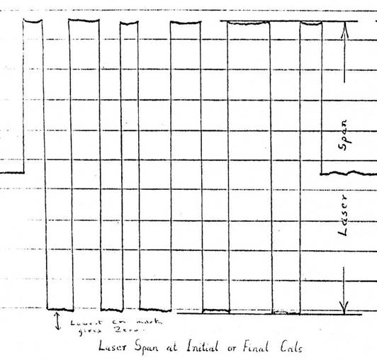
Figure 61 : Example of laser span calibration.
Next, the Barometric Reference Unit (BRU) calibration data was extracted and recorded on the Chart Breakout Sheet. While only the BRU procedure is detailed the procedure was the same for extracting and calculating the calibration constants for the Statoscope. For each BRU calibration pulse, a line was drawn joining the unpulsed trace at the beginning and end of each pulse and a parallel line joining the pulsed trace at the beginning and end of each pulse. The pulse height was then measured in millimetres, perpendicular to the chart’s grid lines between the two drawn parallel lines, please refer to the example at Figure 62. For both the BRU and Statoscope units the pulse height varied with flying height. WRE had compiled a set of empirical tables for both units which gave the pulse height, in metres, for a given flying height. The average BRU pulse heights extracted from the chart was around 20 millimetres. At nominal flying height this represented some 12 metres of height change. Thus, the BRU ratio was usually around 1 millimetre on the chart indicating 0.6 metres of height change by the aircraft at that altitude. As the aircraft could climb or descend during a line the displacement of the BRU trace could be either positive or negative. To ensure that the appropriate BRU correction was applied for the aircraft’s departure from the starting pressure surface, the BRU trace was output such that it rose as the aircraft descended and vice versa. Thus, as the aircraft descended and the aircraft to terrain distance was reduced the positive correction as given by the rising BRU trace correctly adjusted the extracted height for the aircraft’s departure from the atmospheric datum.
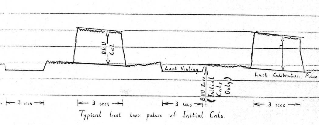
Figure 62 : Example of BRU calibration.
The Vertical Roll Gyro (VRG) trace indicated the amount of aircraft movement from level flight. Initially, the trace was only used to indicate where the aircraft’s movement meant that the laser was not vertical to the terrain and any heights obtained in that region were false. As the gyroscopes became more reliable a start and end calibration was attempted but it was found that this technique introduced greater error into the final heights than totally disregarding the gyroscope. From about 1973 as part of the installation and testing process the gyroscopes output on the chart was assessed against a known bank angle of the aircraft. The sea off Adelaide provided a flat surface so that any movement of the aircraft from the vertical would mean a dip in the laser profile trace could be observed on the chart. No matter if the aircraft rolled left or right the aircraft to sea level distance would increase and this increase would be shown on the chart as though the terrain was falling away. This fact meant that any correction due to roll was always positive. As the aircraft was never rigidly stable with respect to the terrain, an unobservable amount of roll was always present. To account for this occurrence all final heights from 0.5 and above were always rounded up to the next whole unit.
To determine the relationship of roll angle to chart displacement of the gyroscope trace, after flying straight and level at the nominal flying height of 7,000 feet, the pilot would slowly induce a known bank angle of say 5 degrees and after stabilising at that angle of bank for a few seconds slowly return to straight and level flight again. Only angles up to 10 degrees, being both left and right roll angles, were tested. The chart now showed the departure of both the roll gyroscope and laser profile trace from the vertical to the known roll angle. The theoretical correction for that altitude and roll angle could also be calculated. The discrete values obtained inflight could thus be used to modify the theoretical values and allow the interpolation of corrections for intermediate roll angles. The departure of the roll gyroscope trace in millimetres on the chart for a discrete roll angle could also be used to interpolate the departure in millimetres on the chart to intermediate roll angles. Ultimately a graph could be drawn such that height correction for roll could be read for any departure in millimetres on the chart of the roll gyroscope. This graph however was only valid for the aircraft to ground distance being 7000 feet. The graph was thus enhanced to be able to read the roll correction for a common range of aircraft to ground distances.
It was also found that it was more accurate to determine the departure from level flight around the region of the chart where the departure had occurred. Hence the term Take local Zero being entered on the Chart Breakout Sheet.
If circumstances permitted all the above was done in the field and the completed and checked Chart Breakout Sheets were freighted back to the office with the other materials.
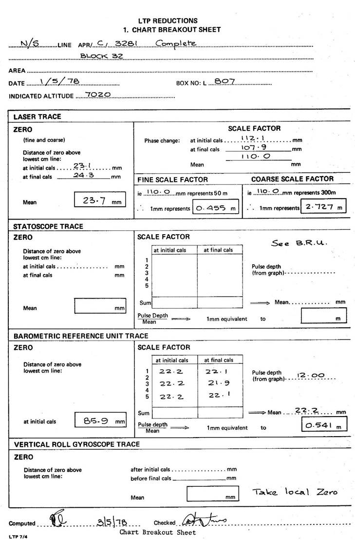
Figure 63 : Example of a Chart Breakout Sheet.
Relating each profile chart to AHD and height reductions
The process to determine the AHD height for each point in a photogrammetrical model from a profile chart started with the north-south tie lines being related to the bench marks which were specifically overflown during the profiling of these lines. The ground control generally bench marks was already based on the Australian Height Datum.
As the profile rarely passed exactly over the particular ground control, the absolute height of the profile was found by selecting a point or points on the terrain profile near the ground control and reading their relative height differences at 1: 80,000 photoscale in a photogrammetric plotter. All control points were related to the adjacent profile in this manner. Simplistically, now that two points on a continuous terrain profile had known values, adopting the AHD elevation of the first point on the profile, the elevation of the second point could be calculated from the chart. The difference between the chart value and the actual AHD elevation of the second point was the misclose. This difference could be linearly proportioned along the profile and applied to any intermediate point. The difference between the known AHD height at the first point and its chart value was called the Fine Zero for that chart.
With the north-south tie lines now being related to AHD, each of the east-west profiles could be processed as they intersected a tie line at their beginning and end. The intersection points were found from the 70mm positioning photography and transferred to the respective chart via the time code. The AHD value for the start and end of the east-west profile was calculated from the applicable tie lines. Again, at the start point, the difference between the known AHD height at that point and its chart value was called the Fine Zero for that chart. The AHD value of the end point was calculated from the chart and compared with that from the tie line value. Any misclose was again linearly proportioned along the east-west profile and applied to any intermediate point. Thus, for any point along any terrain profile an AHD value could now be extracted.
Using the information in Figure 64, the following explains how a height required at the film time extracted as 3 hours 10 minutes 5.8 seconds was obtained. From the chart timecode this point is identified as point P in Figure 60.
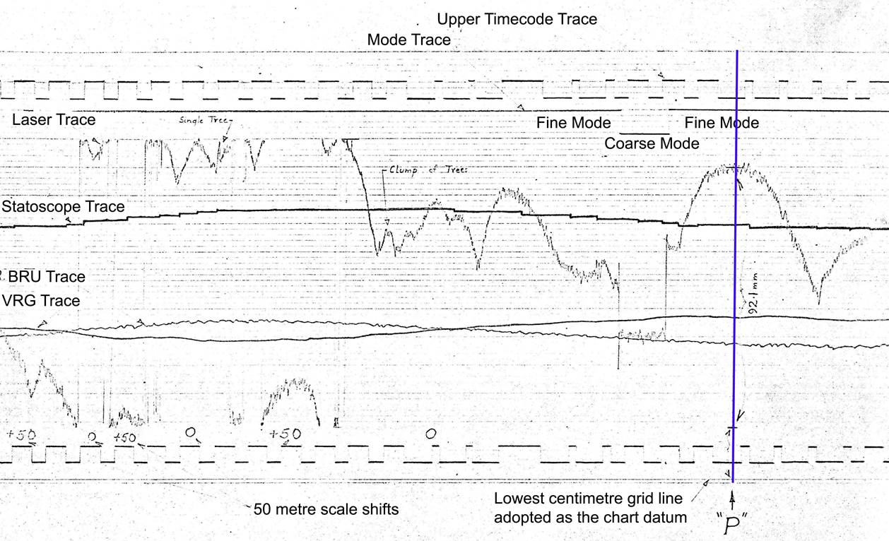
Figure 64 : Section of a laser profile chart for which the height of point P is determined to show the steps involved.
At point P in Figure 60, the distance of the laser trace above its chart datum, as given in this Chart’s Breakout Sheet, is measured as 92.1mm above its calibrated zero value of 23.7mm. Similarly, the BRU trace at point P is measured as -5.6mm below its 89.5mm Chart Breakout Sheet calibrated zero distance. Also at point P, it is assessed that there is 2.3mm of aircraft roll. Figure 65 is an example of the LTP Reduction sheet in which for point P the time of 3h10m5.8s and chart measurements of 92.1mm, -5.6mm and 2.3mm have been recorded. Also at point P, a scale shift of 0 (zero) is recorded. The Corrected Chart Height was then calculated by converting the respective chart distances in millimetres to meters by multiplying them by their factor as determined in the Chart Breakout Sheet and adding the three results together arithmetically; giving 39.2 metres in the example.
The Fine Zero and misclose for this chart and point were determined separately at 421.1m and -7.8m respectively as shown below. The Corrected Chart Height of 39.2m plus the Scale shift of 0m plus the Fine Zero value of 421.1m are arithmetically combined to give the Absolute Chart Height for point P of 460.3m. The Absolute Chart Height for point P of 460.3m is lastly corrected by the misclose of -7.8m to 452.5m.
All chart measurements were to 0.1 millimetres and heights were calculated to 0.1 metres and rounded up to the next metre. Rounding up was adopted as explained, as any undetected aircraft roll will indicate a height that is lower than true on the laser trace. Thus, the final height for point P is determined as 453m.
|
LTP REDUCTIONS Page 1 of several |
|||||||||||||||
|
APR/C/3281 |
|
6. HEIGHT LIST |
|||||||||||||
|
|
|
|
FINE ZERO = 421.1
|
Laser Fine Zero |
23.7 |
mm |
|||||||||
|
AREA Block 32 |
Laser Scale Factor |
0.455 |
|
||||||||||||
|
Date Flown 1/5/78 |
|
||||||||||||||
|
ALTITUDE 7020 |
BRU/Stato Zero |
85.9 |
mm |
||||||||||||
|
Box No. LTP807 |
BRU/Stato Scale Factor |
0.541 |
|
||||||||||||
|
|
|||||||||||||||
|
1 |
2 |
3 |
4 |
5 |
6 |
7 |
8 |
19 |
10 |
11 |
12 |
|
|||
|
Point No. |
Timecode |
LASER |
BRU/Stato |
V.R.G |
Cor. Ch. Reading (3+4+5) |
Scale
Shift |
Absol. Ch. Height ((6+7+FZ) |
Misclose
(from gr.) |
HEIGHT
(meters) |
FINAL
HEIGHT |
REMARKS |
|
|||
|
Mm |
M |
Mm |
M |
mm |
M |
|
|||||||||
|
P |
3h10m5.8s |
92.1 |
41.9 |
-5.6 |
-3.0 |
2.3 |
0.3 |
39.2 |
0 |
460.3 |
-7.8 |
452.5 |
453 |
|
|
|
|
|
|
|
|
|
|
|
|
|
|
|
|
|
|
|
Figure 65 : A sample calculation showing the chart data being reduced to a terrain height.
The LTP Reduction form, as shown in Figure 66 below, was originally designed in an era when only mechanical calculators were available. Thus, each step or combination of steps could be easily recorded. Even though basic and then programmable hand electronic calculators became available over time this sheet layout remained unchanged as it immediately showed where any error occurred. As all the above processes were manual, each step was independently checked and being able to immediately see a mis-measurement or -recording saved time.
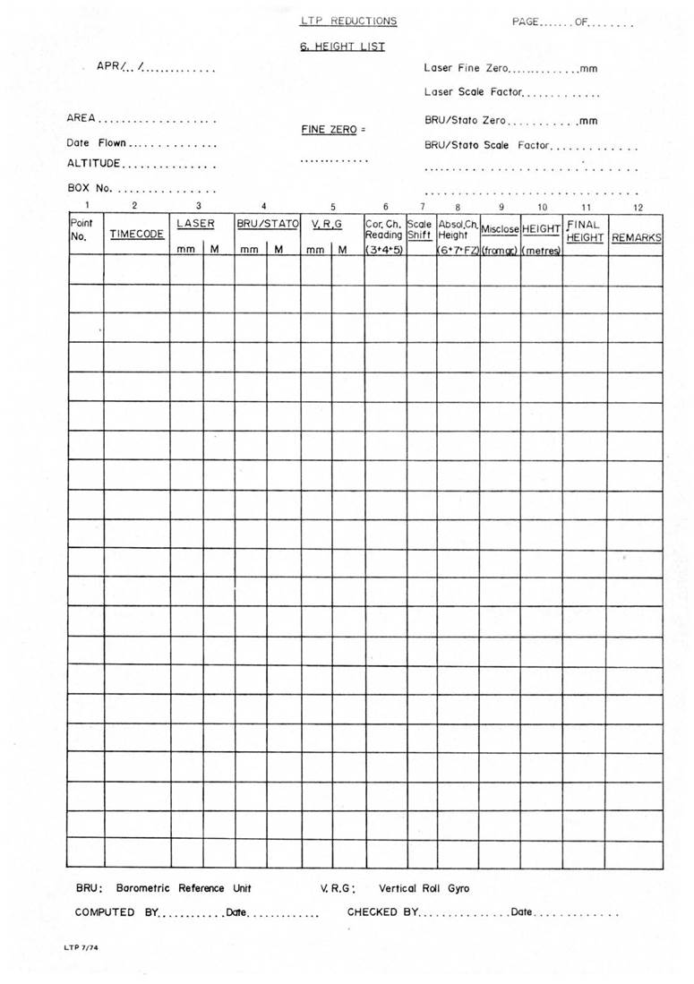
Figure 66 : Sample LTP Reduction form.
Quality checks and accuracy
The laser measured the distance to an accuracy of ±0.3 metres at all times. However, cumulative errors due to the dependence on a barometric reference to measure aircraft displacement from an isobaric surface, which was not always stable, and the tilts of the aircraft, could sometimes decrease the accuracy of heights extracted from the laser profiling system, to ±3 metres. In practice, an accuracy of ±2 metres was expected.
In the early 1970s, the first photogrammetric checks were applied to the heights of points extracted from laser terrain profiles over eight 1: 250,000 scale map areas, representing a wide variety of terrain from flat to mountainous country. These checks were obtained by photogrammetrically levelling photogrammetric models, containing published Australian height datum ground control, solely on the heights of the laser points, then reading the differences to the ground control within the models. The results of the 451 photogrammetric height comparisons showed 63 per cent of the heights were within 1 metre, 86 per cent were within 2 metres, 95 per cent were within 3 metres, 99 per cent were within 4 metres and 100 per cent were within 5 metres. In such a comparison the fact that the pointing accuracy of the photogrammetric restitution instruments used for levelling the 1: 80,000 scale aerial photography models was of the order of ±1.5-2.0 metres, needed to be appreciated.
It was thus considered that as the accuracy of the heights derived from the laser terrain profiler and the photogrammetric restitution instruments used for plotting contours from the 1: 80,000 scale aerial photography models were of similar magnitude the two systems were compatible.
As a final check on the quality of the heights produced from the terrain profiles for each 1: 250,000 scale map sheet area, selected profile heights were photogrammetrically compared to ground control not used previously in controlling the tie lines for the area. Photogrammetric models containing the extracted profiler heights and existing control were placed in a stereoplotter and oriented as for contour generation. The stereoplotter height was noted for each of the known ground control points and compared with their actual values. Any point with a residual larger than 5 metres was investigated and, in most cases, resolved. The final height lists, aerial photographs and diapositives were then approved for use in subsequent stereoplotting and contouring.
Annexure I shows Nat Map’s completed laser terrain profiling by calendar year from 1970 to 1975 and 1977 to 1979.
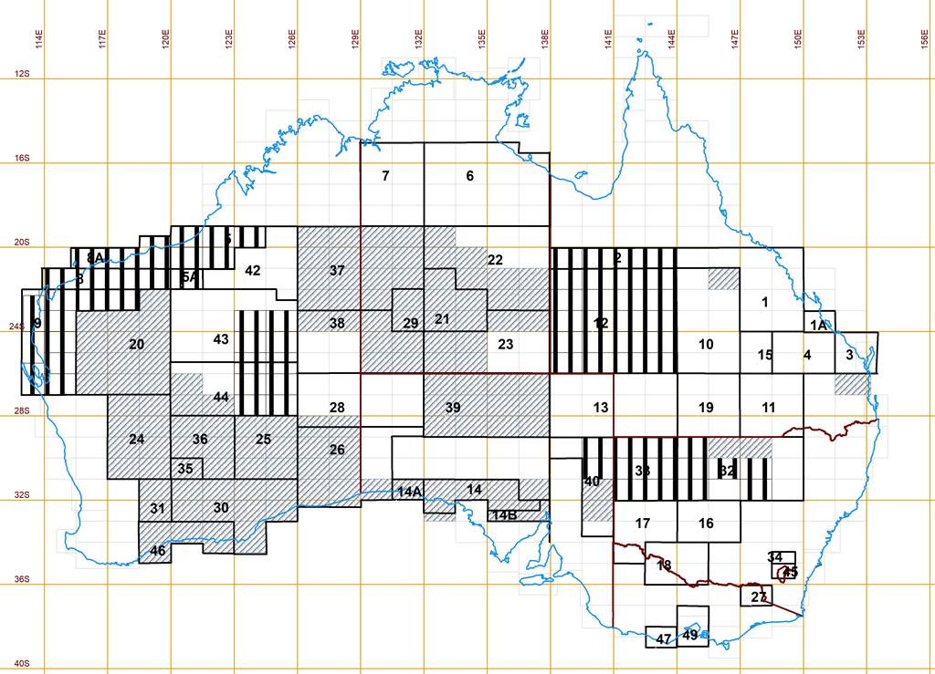
Figure 67 : Map showing the 1: 250,000 scale map areas where laser terrain profiling was completed between 1970 and 1975 in VH-EXP.
The vertical stripes show the map areas where laser terrain profiles were flown to strengthen the original APR profiling.
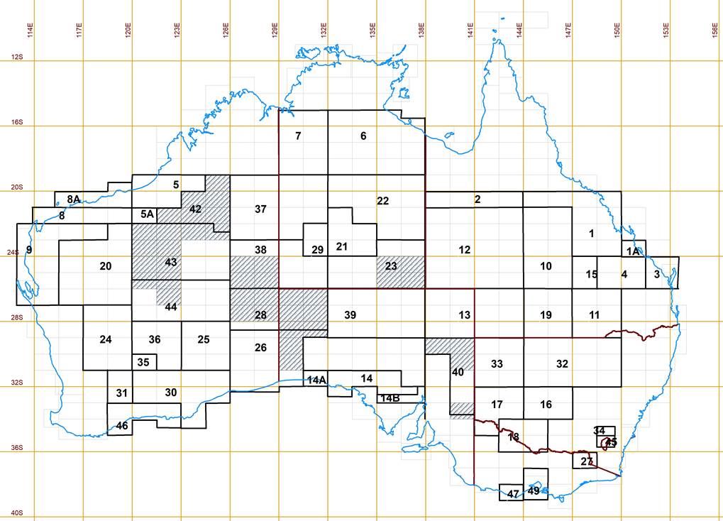
Figure 68 : Map showing the 1: 250,000 scale map areas where laser terrain profiling was completed between 1977 and 1979 in VH-DNM.
Other Projects involving the Nat Map Laser Terrain Profiler
Proposed Tarcoola-Alice Springs rail route
In 1970, when Nat Map’s profiling operations were based at Alice Springs, profiles along the then proposed Tarcoola-Alice Springs rail route were acquired. While the concept was sound, and indeed the results could have had a significant positive impact on the project’s route planning, the work was ultimately unusable. The problem was that at that time the region only had 1: 250,000 scale R502 series mapping and had not been captured as part of the aerial photography program. Thus, there was no way to accurately relate the location of the profiles in the terrain. Without accurately knowing where the profiles had been acquired any height information that could have been extracted, was useless. Nevertheless, the experience was invaluable and no future profiling was undertaken prior to recent aerial photography already being available.
Microwave Repeater Station siting and design
At the request of the then Post Master General’s Department (PMG), in 1973 laser profiles were acquired to assist planning the locating of Microwave Repeater Stations. The routes were Port Hedland to Wittenoom in the Pilbara region of Western Australia and Cairns to Bamaga across Cape York in Queensland. While the high points in the terrain were obvious sites for the microwave towers what was required was a profile of the intervening terrain. These profiles would help determine the final tower heights and placement for optimum transmission and reception. In both cases the harsh remote desert and tropical jungle made obtaining this data by ground methods complex and thus expensive.
Before any flying was undertaken the PMG’s engineers had established and marked (to be visible from the air) the high points for possible tower siting and likely tower to tower paths. On a couple of paths intermediate sites were marked in case the most direct route proved unusable. The PMG’s engineers required profiles of all paths and these would be provided by Nat Map in the form of scaled graphical plots of the terrain from site to site showing the lowest point(s) and any specific obstacles.
The positions of the marked tower sites were transferred to navrolls and the required paths then established. As the profile was required to be the direct tower to tower route turning of the aircraft once on line had to be avoided. It was thought that if possible the aircraft should be aligned, allowing for drift, hill top site to hill top site. This proved to be much more difficult operationally such that the required paths were profiled in both directions and the profile(s) best meeting the requirements then selected for use and supply to the PMG.
Map Accuracy
A check on 1: 100,000 scale (20 metre contour interval) orthophoto maps in Queensland, which had been compiled using radar terrain profiling for height control, was performed in the early 1970s. From a terrain profile of 36 kilometres, the heights of 24 contour crossings were extracted and compared with their contour value. The standard deviation between the orthophoto and laser profile heights was 2.6 metres, with a maximum deviation of 4.4 metres, which indicated compatibility between radar and laser profile derived heights for mapping projects at 1: 100,000 scale.
Over a forested, mountainous area, a comparison of the ground profile as determined by the laser profiler with 1: 9,600 scale mapping, was undertaken. From a terrain profile of 8 kilometres, the heights of 16 points were extracted and compared with their map value. The height data had a standard deviation of 2.8 metres and a maximum deviation of 6 metres. The laser profile, when plotted against the profile derived from the map contours, illustrated a very close agreement between the respective profiles, even where the terrain was very steep and covered with timber
Later in the early 1980s a number of profiles were flown across selected 1: 100,000 scale map sheets to check that their vertical accuracy met the 1: 100,000 scale map specification. These map sheets were mainly in Victoria.
Operation Desert Walk 80
In March 1980 Nat Map acquired profiles for the Royal Australian Survey Corps as their WREMAPS2 system was inoperative. The project was named Operation Desert Walk 80 and was for the production of 1: 50,000 scale topographic maps in the Maralinga area of South Australia.
Laser Terrain Profiling Finale
At a small ceremony at noon on Thursday 9 September 1982, the last laser chart had the data for a number of points symbolically extracted by those who had worked on the laser terrain program over the years. Figure 65 shows the areas of Australia where terrain profiling by APR and LTP was acquired between 1962 and 1979; Figures 63 and 64 above show the areas profiled with the LTP system installed in the Grand Commander VH-EXP and the Nomad VH-DNM, respectively. Figure 66 is a photograph taken during the informal ceremonies of 9 September 1982.
The laser terrain profiling program’s significant events and statistics were :
|
Date |
Event |
Notes |
|
Tuesday 18 August 1970 |
First program line flown near Broken Hill |
Rom Vassil, John Ely, Terry Mulholland |
|
Thursday 6 December 1979 |
Last program line flown near Giles |
Paul Wise, Ozcan Ertok, Andrew Hatfield, Harry Baker (Pilot) |
|
Tuesday 1 April 1980 |
Last actual line flown near Forrest |
Rod Menzies, Ozcan Ertok, Bob Goldsworthy, Peter Prior (Pilot) |
|
Thursday 9 September 1982 |
Last heights extracted |
|
|
|
||
|
Other statistics |
|
|
|
Line kilometres flown |
250,000 - about 6 times around the globe |
|
|
Charts used |
1200 - about 60 kilometres |
|
|
70mm film used |
800 - about 8.5 kilometres |
|
|
|
|
|
|
Vertical Control |
|
|
|
Points selected |
50,000 but probably triple that number when control and check points included |
|
|
Area (map sheets) |
172 - 1:250 000 scale map sheets |
|
|
Area (square kms) |
2.7 million - mainland Australia is 7.7 million square kilometres |
|
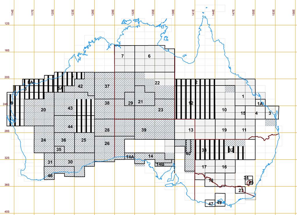
Figure 69 : Areas of Australia where terrain profiling by APR (light) and LTP (heavy) was acquired between 1962 and 1979.
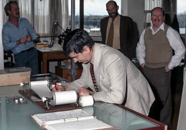
Figure 70 : Photograph taken by Adrian Wright on Thursday 9 September 1982 with (L-R) Terry Mulholland, Syd Kirkby and Paul Wise watching Rom Vassil extract a height from the last laser chart.
People involved with the Laser Terrain Profiling program
Such a program is not achieved without the efforts of those involved. When the weather was devoid of high and low cloud, the aircraft was not unserviceable or the pilot out of flying hours, the equipment was not hampered by leaky lasers, modulator bubbles and electronic gremlins, the personnel including navigators were not getting lost, camera operators not jamming cassettes and technicians not blowing capacitors, and further there was no turbulence, cross winds or hail, fuel drums were not disappearing, nor refuelling pumps leaking, nor airport refueler refuelling difficulties and the late nights and early mornings were not affecting the parties mental state, then successful airborne terrain profiling operations occurred. Strangely in hindsight, all the above instances, while remembered for their frustrating impact at the time, were in the minority and for the most part terrain profiling operations were routine. Some Natmappers only worked on the office side of the program extracting the height information from the charts. This mundane work was of no less importance and their efforts should be applauded equally with those who undertook the more visible field activity.
The contract pilots who flew VH-EXP and later VH-DNM should also not be overlooked. Some had already experienced flying with Aerodist and so working with Nat Map was nothing new. To other pilots however, the experience was new but within days most had assimilated and flying operations continued almost seamlessly. What part the very astute management of Executive Air Services played in ensuring only pilots who could and would be easily assimilated into Nat Map’s field parties were sent, is unknown.
To those who worked on the laser profiling program either in the field or office they were part of an era that with the technological advancement will never be repeated. As best as records and memory will allow, those listed below all played their part.
|
Senior Supervisory Staff |
|
|
Joe Lines |
|
|
Len Turner |
|
|
Syd Kirkby |
|
|
Bob Bobroff |
|
|
Rom Vassil |
|
|
Andrew Turk |
|
|
John Manning |
|
|
|
|
Field Party Leaders |
|
|
Norm Edwards |
|
|
Simon Cowling |
|
|
Paul Wise |
|
|
Rod Menzies |
|
|
Mike Morgan |
|
|
Bruce Hewitt |
|
|
Ian Hall |
|
|
Martin Kros |
|
|
Peter Quinn |
|
|
Carl McMaster (PRAM/LAPS) |
|
|
Ed Burke (PRAM/LAPS) |
|
|
|
|
Electronics Technicians |
|
|
Ozcan Ertok |
|
|
John Ely |
|
|
Mick Skinner |
|
|
Terry Mulholland |
|
|
Des Fahey |
|
|
Andrew Christie |
|
|
Arnold Visser |
|
|
Donald Sutherland |
|
|
|
|
Strip-camera Operators/Bookers |
|
|
Adrian Wright |
|
|
Graeme Lawrence |
|
|
Andrew Hatfield |
|
|
Ian Graham |
|
|
Bill Stuchbery |
|
|
John Corcoran |
|
|
Ross Chisholm |
|
|
Julie Gould |
|
|
Leon Derkacz |
|
|
Dave Henderson |
|
|
Michael Lloyd |
|
|
|
|
Logistics |
|
|
Laurie Edebohls |
|
|
Dave Abreu |
|
|
Reg Kearns |
|
|
Hayden Reynolds |
|
|
Ken Brown |
|
|
John Guilfoyle |
|
|
Peter James |
|
|
|
|
Airstrip preparation & fuel support |
|
|
Laurie McLean |
|
|
Tony Maginn |
|
|
|
|
Fuel support |
|
|
Bob Goldsworthy |
|
|
Roy Turner |
|
|
|
|
Contract Pilots |
|
|
Grand Commander VH-EXP |
|
|
Bob Barnes |
|
|
George Rickey |
|
|
Arthur Johnston |
|
|
Graham Galliott |
|
|
Trevor Merton |
|
|
Dave Leary |
|
|
Pat O’Donohue |
|
|
John South |
|
|
Stan Tayler |
|
|
Phil Robertson |
|
|
|
|
Contract Pilots |
|
|
Nomad VH-DNM |
|
|
Pat O’Donohue |
|
|
Jack Marshall |
|
|
Errol Driver |
|
|
|
|
|
Nat Map Pilots |
|
|
Nomad VH-DNM |
|
|
Harry Baker |
|
|
Peter Prior |
|
|
Terry Mulholland |
|
|
Jock Head |
|
|
|
|
Office only |
|
|
Graham McNamara |
|
|
Apostolos Anagnostou |
|
|
Ed Ainscow |
|
|
Rajanithy (Raji) Nagendiram (later Mrs Ian Muir) |
|
|
Jacqueline Wray-McCann |
|
|
Robert Whitborne |
|
|
Martin Casstanelli |
|
|
Barry Wright |
|
|
Garry Burris |
|
|
Maya Pinkster (nee de Haan) |
|
|
|
Again, as best records and memory will allow, the following is an annual summary of where and who were involved in laser profiling field operations.
|
Year |
Operational Airstrips |
Personnel Involved |
|
1970 |
Broken Hill |
Syd Kirkby |
|
Dubbo |
John Ely |
|
|
Rom Vassil |
||
|
Terry Mulholland |
||
|
|
||
|
1971 |
Mildura |
Rom Vassil |
|
Alice Springs |
Norm Edwards |
|
|
Tennant creek |
Simon Cowling |
|
|
Yuendumu |
John Ely |
|
|
Warrabri |
Des Fahey |
|
|
Charters Towers |
Adrian Wright |
|
|
Graeme Lawrence |
||
|
|
||
|
1972 |
Forrest |
Rom Vassil |
|
Kalgoorlie |
Norm Edwards |
|
|
Meekatharra |
Simon Cowling |
|
|
Carnarvon |
Paul Wise |
|
|
|
Des Fahey |
|
|
Adrian Wright |
||
|
Laurie Edebohls |
||
|
Bill Stuchbery |
||
|
1973 |
Esperance |
Paul Wise |
|
Kalgoorlie |
Mike Morgan |
|
|
Meekatharra |
Mick Skinner |
|
|
Carnarvon |
Oz Ertok |
|
|
Alice Springs |
Arnold Visser |
|
|
Rabbit Flat |
Simon Cowling |
|
|
Halls Creek |
Rom Vassil |
|
|
Cunderdin |
Laurie Edebohls |
|
|
Birdsville |
John Corcoran |
|
|
|
John Guilfoyle |
|
|
Microwave survey : |
||
|
Port Hedland |
||
|
|
Wittenoom |
|
|
Cairns |
||
|
Bamaga |
||
|
|
||
|
1974 |
Esperance |
Paul Wise |
|
Kalgoorlie |
Bruce Hewitt |
|
|
Broken Hill |
Rom Vassil |
|
|
Longreach |
Laurie Edebohls |
|
|
Ceduna |
Oz Ertok |
|
|
Balgo |
Donald Sutherland |
|
|
Dave Abreu |
||
|
Terry Mulholland |
||
|
Ken Brown |
||
|
1975 |
Oodnadatta |
Paul Wise |
|
Alice Springs |
John Ely |
|
|
Vaughan Springs |
Andrew Christie |
|
|
Uluru |
Oz Ertok |
|
|
Reg Kearns |
||
|
Ian Graham |
||
|
Ross Chisolm |
||
|
Tony Maginn |
||
|
Donald Sutherland |
||
|
1976 |
No profiling : VH-DNM replaced VH-EXP |
|
|
|
||
|
1977 |
Alice Springs |
Paul Wise |
|
Fitzroy Crossing |
Rod Menzies |
|
|
Kidson Field |
Oz Ertok |
|
|
Nullagine |
Graeme Lawrence |
|
|
Newman |
Leon Derkacz |
|
|
Meekatharra |
Hayden Reynolds |
|
|
Peter Quinn |
||
|
Peter James |
||
|
Laurie McLean |
||
|
Tony Maginn |
||
|
Bob Goldsworthy |
||
|
Roy Turner |
||
|
1978 |
Forrest |
Paul Wise |
|
Broken Hill |
Rod Menzies |
|
|
Alice Springs |
Ian Hall |
|
|
Giles |
Oz Ertok |
|
|
Uluru |
Mick Lloyd |
|
|
|
Andrew Hatfield |
|
|
Martin Kros |
||
|
Dave Henderson |
||
|
Julie Gould |
||
|
1979 |
Forrest |
Martin Kros |
|
Giles |
Oz Ertok |
|
|
Uluru |
Ross Chisolm |
|
|
Alice Springs |
Mick Lloyd |
|
|
Ian Graham |
||
|
|
Leon Derkacz |
|
|
Paul Wise |
||
|
|
||
|
1980 |
Operation Desert Walk 80 |
Rod Menzies |
|
|
Ceduna |
Oz Ertok |
|
Cook |
Bob Goldsworthy |
|
|
Roy Turner |
||
|
|
|
|
|
Notes : · As personnel were rotated into and out of the field not all personnel listed as being in the field in a given year were there for the whole period. · The bases listed above are shown on the map in Figure 71 below. The Melbourne bases of Essendon and Moorabbin airports as well as the Adelaide bases of Adelaide and Parafield airports were used as required on an annual basis. |
||
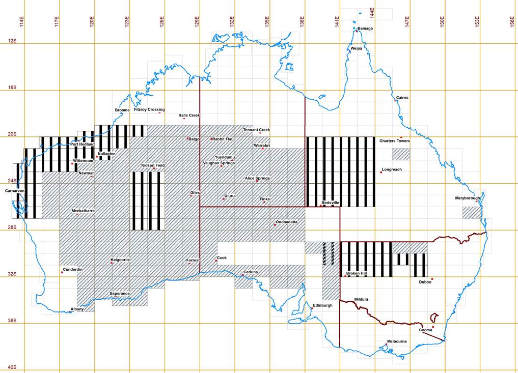
Figure 71 : Map showing bases used by VH-EXP and VH-DNM for laser terrain profiling.
Chapter 6 – National Mapping’s Second Generation Airborne Laser Terrain Profiler
ACCI PRAM to NAT MAP LAPS
With mapping control for the 1: 100,000 scale NTMS program completed, it was foreseen that Nat Map should recompile some of its earliest 1: 100,000 sheets at 1: 50,000 scale. With satellite positioning now available, obtaining any additional horizontal control to meet the 1: 50,000 scale positional accuracy specification would not pose a problem. Obtaining vertical control for plotting contours at a 10 metre vertical spacing was a different matter.
Nat Map was well aware that technology had moved on in the 10 years of WREMAPS1 operation and lasers were now more powerful, compact and efficient and importantly digital output and storage was becoming the norm and thus more reliable. Thus, after researching the options, in the 1984-85 financial year Nat Map acquired a new laser based airborne measuring unit. This unit was integrated, by Nat Map’s own technicians led by John Ely, into a compact, digitally based terrain profiling system. This system operated in Nat Map’s Cessna C421, at Figure 71 below, which had by now replaced the Nomad.
The ACCI (Associated Controls and Communications, Inc. of Cambridge, Massachusetts, USA) PRAM laser was coaxially sited with the original WREMAPS1 70mm strip camera and along with the existing BRU (Barometric Reference Unit) and new control console and data capture system, formed the Nat Map PRAM profiling system. This system later became known as the Laser Airborne Profiling System (LAPS).
The 20pps (pulses per second) YAG transceiver employed a pulsed Nd:YAG (neodymium-doped, yttrium-aluminium-garnet) laser operating at 1064 nanometres with a 10 nanosecond pulse width and 0.5 milliradian beam width. The Model NT-90 Rugged Compact, Nd:YAG laser system was supplied by International Laser System from Florida, USA. Output range of the NT-90 laser was in excess of 20 kilometres, thus more than capable of measuring from 10,000 feet above ground in Australian dust and haze conditions. It incorporated a closed cycle liquid to air heat exchanger with a high capacity, low noise fan to reduce acoustic noise level. Also included was the laser transceiver and control console, including power supplies, associated electronics, nanosecond time interval counter, height computer, control panel, display and interfaces for recording and remote control. An Intel 86/05 single board 16 bit microprocessor performed all mathematical calculations, diagnostics, range gating, computer to computer interfaces, range conversions and had output functions for an RS-232 interface. It was capable of at least ±10 centimetre accuracy in all conditions and all up weighed only 20 kilograms (Jepsky, 1986). The onboard data logger computer initially used was a Hewlett Packard 85 model.
The complete airborne system was designed so that each time the laser pulsed and digitally recorded a height above terrain the location was recorded on the 70mm strip camera and a digital BRU reading was also captured.
Digital capture enabled inhouse developed, computerised post processing, eliminating the previous, tedious and error prone, manual height point determinations previously described.
The location of height points was digitised from the strip film and immediately related to their relevant raw data by the computer. In addition, any correction provided by the BRU could be applied as well as misclose correction provided by relating appropriate profiles to AHD bench marks, thus delivering the final heights on AHD. The airborne and office components of this system are shown in Figure 73 below.
|
|
|
|
Figure 72 : Natmap’s aerial survey platform Cessna 421, VH-DRB |
|
|
|
|
|
Operator’s console in Cessna 421 |
Laser and receiver in Cessna 421 |
|
|
|
|
Ground profile recorded on 70mm film related to profile by timecode |
|
|
|
|
|
Digitiser input |
Profile display |
|
|
|
|
Computer controller and input |
|
|
Figure 73 : Photographs of the airborne and office components of the initial LAPS system. |
|
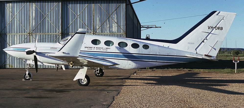
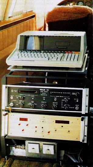
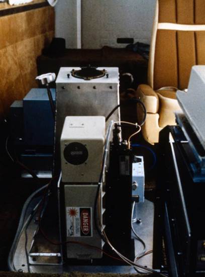
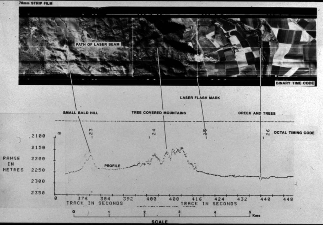
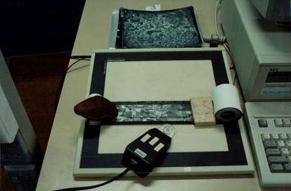
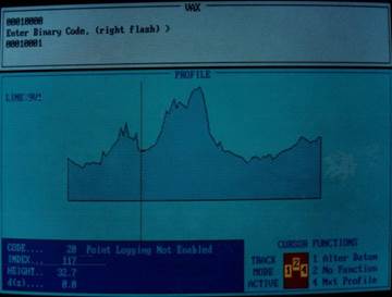
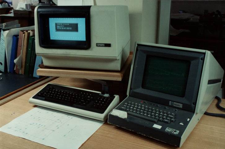
Following initial profiling operations in Queensland in 1985 the system was upgraded to include the following :
|
· |
David Digital Elevation Computer (replaced the BRU) |
|
· |
Computer Buffer for data logging system (128 kilobytes) |
|
· |
NEC APC IV Powermate I Personal Computer with 1.2 Mbyte and 0.7 Mbyte floppy disk storage (replaced HP85 as data logger) |
The system specifications were now as follows :
|
Laser |
|
|
NT-90 |
50mJ Nd:YAG Laser |
|
Pulse energy |
50 mJoules |
|
Pulse width |
10 nanoseconds |
|
Beam divergence |
0.5 milliradians |
|
Beam width at source |
38 millimetres |
|
Wavelength |
1064 nanometres |
|
Ground pulse width from 10,000 feet above terrain |
1.2 metres |
|
Repetition rate |
5/20 pulses per second (user selected) |
|
Strip Camera |
|
|
Focal length |
88.9mm |
|
Format |
70mm |
|
Capacity per cassette |
23 metres |
|
Total number of cassettes |
4 |
|
Each cassette is equivalent to 710 kilometres @ 9,000 feet above terrain @ 360 kilometres per hour ground speed |
|
|
Disk Storage |
|
|
File length limited to 1.2 Mbyte, maximum line length at 20pps limited to approximately two hours continuous operation in the aircraft. In practice the lower 5pps option is used away from intersection or ground control points generating a profile measurement at about a horizontal interval of 20 centimetres. |
|
|
LAPS weight |
|
|
Total 130 kilograms |
|
|
Aircraft Requirements |
|
|
24-28 volts, 15-20 Amps
|
|
Henry Correction Reimagined
With the acquisition of the new laser terrain profiling system and the need to ensure that the height information it would be producing would meet 1: 50,000 scale map accuracy standards, Nat Map’s terrain profiling methodology underwent a review.
As described above, Nat Map’s new laser terrain profiler had been purchased to ensure that when operated in Nat Map’s Cessna C421 at 10,000 feet ASL in Australian conditions, it would meet its quoted accuracy of at least ±10 centimetres. Nevertheless, final height accuracy would still depend on using the isobaric surface. It was anticipated however, that now being able to fly faster and at 10,000 feet the atmospheric conditions would remain more consistent during the period of terrain profile acquisition. Consistent conditions would mean that many of the small, unnoticeable variables would be removed rather than accumulate and impact the final result.
By now Nat Map also had the computing power to undertake its photogrammetric block adjustments by analytical or numerical methods. Nat Map’s slotted template method of photogrammetric block adjustment had at last been overtaken by technology! As explained above, the analytical or numerical approach to control intensification meant that Nat Map now acquired its terrain profiles in an almost square grid pattern with a spacing of about 60 kilometres. In addition, terrain profiles were acquired along the perimeter of the photogrammetric block. This spacing of terrain profiles had been determined by the block adjustment’s minimum requirements for vertical control. There had never been an assessment as to whether a narrower spacing between terrain profiles might improve the heights derived from these profiles. To meet 1: 50,000 scale map accuracy standards, Nat Map had to now have a high degree of certainty that heights extracted from its terrain profiles to produce 10 metre contours were accurate to ±5 metres or half the contour interval.
The underlying assumption in the analysis was that the adjustment of the terrain profiles to existing vertical ground control would eliminate all errors associated with using a barometric datum. In reality this could never happen as the variables have various errors which could not be detected. It was the impact of these undetectable errors and how they could be reduced or at least minimised that was the aim of the analysis.
Using a baseline set of indicative or accepted variables, the Henry correction was calculated for a theoretical terrain profile flight. Next by recalculating the Henry correction with the variables independently and cumulatively having introduced errors that could have occurred during the flight, it could be observed how those errors impacted the Henry correction value. In theory, during the adjustment of the terrain profiles to existing vertical ground control the baseline value for the Henry correction would be adjusted to be zero. Any departure therefore from the baseline Henry correction value caused by the various introduced errors could be regarded as an indicator of accuracy of the final heights extracted from the applicable profile.
As the maximum error was being assessed, all the variables were taken as being positive although in practice they were likely to be a mix of positive and negative. The analysis is detailed at Annexure J.
The initial analysis was based on having terrain profiles spaced at 60 kilometre intervals. From this initial analysis it was seen that whereas latitude and True Air Speed misinterpretations had little effect on the outcome, misinterpreting drift and time were such that when combined they caused a maximum error of ±2.7 metres compared with the value of ±3.0 metres obtained when all factors were considered. Given that the accuracy requirement for 1: 50,000 scale 10 meter contours was for heights to be within ±5 metres a combination of inflight variables might result in the ±5 metre limit being exceeded.
A second analysis was thus performed adopting 30 kilometres as the spacing between terrain profiles. In addition, a larger drift angle was adopted to see the effect of the higher value which could occur from time to time in terrain profiling operations. Despite the higher drift angle used, the total error of ±2.2 metres was now less than half that of the ±5 metre requirement for 10 metre contouring. With terrain profiles spaced at 30 kilometre intervals to now exceed the ±5 meters requirement a blunder with either drift or time would have to be made. Such an event was highly unlikely given that the values for these two variables have expected bounds and approaching or worse exceeding those bounds would immediately demand a double check.
It was the conclusion of this investigation that the spacing between terrain profiles should be reduced to around 30 kilometres for profiling with the PRAM system installed in Nat Map’s Cessna 421. Such a spacing between terrain profiles should guarantee that the final heights obtained from the terrain profiles were suitable for generating 10 metre contours for 1: 50,000 scale mapping.
Operations
In operation the PRAM module measured the time interval between laser pulse transmissions and reflected ground returns to provide ranging information in electronic and visual form on a LED display. A time reference was used to correlate system ranging data with the Digital Elevation Computer and to generate the flashing of a binary time code onto the strip camera’s film. A marker indicating every 20th pulse was also shown on the film. Information from the Digital Elevation Computer was logged every second of time and each laser pulse return was individually logged. The file length in the NEC personal computer was limited to 1.2 Mbytes permitting a maximum profiling length at 20pps of about two hours continuous operation before it was necessary to download the stored data.
Aircraft navigation was by visual techniques using a Wild NFK2 driftsight and planned flight lines were drawn on aerial photography or Landsat imagery. Vertical control for each 1: 250,000 scale map sheet usually consisted of 6 or 7 north-south profiles and two east-west profiles, one at the top and bottom of each area. Where possible flight lines were planned to pass over existing bench marks. Output from the profiling, apart from the real time LED display on the PRAM module, was fully digital.
Data Reductions
The validation and calculation of profiles along individual flight lines was carried out on the NEC Powermate 1 personal computer with the aid of a Houston 8011 digitising tablet and a Hewlett Packard Quietjet Printer.
Verification and initial processing of data was carried out in the field. Personal computer software had been compiled in Turbo Pascal to capture (DATCAP), verify (V-STRIP) and adjust the profile data generated by the profiler and Digital Elevation Meter. A least squares adjustment of the network intersections and fit to all ground control was carried out on the office VAX 11/750. Using the strip film, selected points were stereoscopically transferred onto the mapping photography for observation in the aerotriangulation process.
Results
Profiling again largely depended on a number of factors such as weather, aircraft operational constraints, profile configuration, vegetation, and type of country. System accuracies were affected by slope of the terrain, foliage reflectance of the ground, turbulence, instability in the isobaric surface.
In 1987/88 two projects were undertaken as part of the 1: 100,000 scale map revision program, upgrading the original radar profiles flown twenty years before. Please refer to Figure 74 below. The first was a block of three map sheets, Mount Coolon, Mackay, St Lawrence, and the second a block of six map sheets from Springsure to Roma. In this terrain profiling survey 7,500 line kilometres were flown over a period of five weeks. On one good day 1,500 kilometres were flown during a 6 hour period. On this work the Cessna 421C operated at a ground speed of 360 kilometres per hour at an altitude of 3000 metres.
A least squares adjustment program (LASADZ) was used to adjust the laser network. This incorporated an interactive solution which employed robust estimations and gross error detection (DANISH). The final adjustment for the southern block of six sheets was run on 10 October 1988. The maximum residual in ground control was +2.9 metres and the maximum residual in line intersections was +2.4 metres. These results were assessed as having a height accuracy of 2 to 3 metres, sufficient for 10 and 20 metre contouring for the analytical aerotriangulation block.
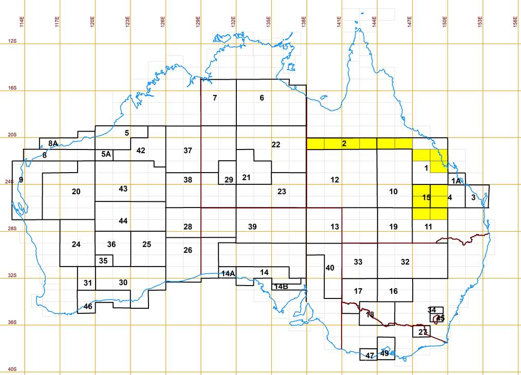
Figure 74 : Map showing the 1: 250,000 scale map areas where PRAM/LAPS terrain profiling was completed in Cessna 421, VH-DRB.
Indonesian Operations
The LAPS was contracted to the private Canadian firm McElhanney Group Ltd for profiling work in Indonesia. The mapping work in Indonesia was part of the Resource Evaluation and Aerial Photography Project (REAP) began in 1978 under a loan agreement between the Governments of Canada and Indonesia. In 1987 the loan agreement was amended to convert the remaining amount of the agreement to grant funding. The purpose of the project was to provide basic materials and data to allow the Indonesian government to properly and accurately evaluate, assess and plan the development of their natural resources on the islands of Java, Sulawesi, Kalimantan, Bali, Madura, and the Nusatenggaras through the establishment of ground control, the production of aerial photographs and the provision of necessary tools, technical assistance and training and techniques.
The project was divided into three phases: (I) the establishment of horizontal ground control; (II) the acquisition of mapping quality aerial photographs; and (III) the development of and the provision of vertical control data, aerial triangulation and numerical adjustments to allow the production of accurate and sufficiently detailed topographic maps to meet the resource development needs of the Republic of Indonesia.
Prior to 1986 the first two components of the project were completed, leaving the third component to be carried out over the Islands of Kalimantan and Sulawesi. McElhanney Geosurveys Ltd carried out Phase III in 1989 using LAPS. Bakosurtanal acted for the Indonesian government in the supply of material and administrative arrangements. LAPS was provided along with technical support and installed in aircraft in Indonesia.
The End of National Mapping’s Airborne Terrain Profiling Operations
The Government’s Administrative Arrangements of July 1987 saw the merger of Nat Map with the Australian Survey Office (ASO) within the Department of Administrative Services (DAS) to form a new entity, the Australian Surveying and Land Information Group (AUSLIG). Nat Map’s Dandenong office thus became part of AUSLIG’s Victorian Regional Office and base for LAPS. In line with other DAS agencies, AUSLIG was required to act as a business enterprise and cost recover its activities including any airborne terrain profiling. In the early 1990s this requirement led to a major reduction in the size of AUSLIG and considerable tension with the private sector. Following a further review in 1996, the Government sold the commercial component of AUSLIG including LAPS. On return from its contract work in Indonesia it is understood that LAPS undertook no further airborne terrain profiling work and eventually passed into obsolescence.

Figure 75 : (L-R) Ian Graham and John Ely with their Department of Administrative Services, Award for Excellence certificates.
Despite its brief operational existence, the development of LAPS was recognised by the then Department. On Wednesday 11 July 1990, Harvey Jacka, the Executive General Manager of the Property Services program of the Department of Administrative Services presented Ian Graham and John Ely with Award for Excellence certificates. Please refer to Figure 75 above. The award recognised their contribution to the development of LAPS. In accepting their awards, both John and Ian said that their awards were a reflection of the work done by many staff on the system development.
Chapter 7 – Then there was the time…
whilst profiling adjacent to the Queensland coast the urge to see the nearby offshore island resort became too great. At the end of a line the flight was extended to include a couple of low passes down the beach and a circuit of the island which gave the crew a great view of the resort and likewise those at the resort could not help but notice the aircraft. One of those holidaymakers just happened to be Natmap’s Director who was quickly on the phone seeking an urgent Please explain from the party leader!
the capability of our Nomad was demonstrated at Ceduna when a fairly new (to the aircraft) pilot wanted to practice a short field landing. He put the plane down on the start of the piano keys and stopped before we reached their end - admittedly there was a bit of a headwind.
when the hire car at Meekatharra had its four wheels stolen during the night so that the next morning as we were about to leave for the airport there was our vehicle sitting of four stacks of bricks!
at Nullagine when we had to report the possible theft of 44 of our empty then 44 gallon drums of AVTUR (AViation TURbine Kerosene) from the airport. In haste the aboriginal police constable was told 44 of our 44’s have been taken! He visibly paled as he looked up fom his report sheet and asked What were you doing with so many guns?
when flying profiles out of Nullagine, where we would fly a line east to the WA/NT border (about 4 hours) then refuel at Kidson Field (a dirt strip put in near the Canning Stock Route for oil search operations). We would then fly another line east back to Nullagine. At the end of the first flight of our section of the survey, the pilot and navigator found that both were new to the area and also found that Kidson was not marked on any charts; being low on fuel that was a problem. The ground crew at Kidson, when contacted, couldn’t hear any aircraft. A check of maps and photos revealed some areas devoid of sandridges and likely to be the site of the strip. Heading towards the most likely area, thankfully the ground crew heard the aircraft and guided us in. The first job, before having the roast lunch that was awaiting us, was to mark Kidson on every available chart and photo. While the flight crew ate lunch the ground crew refueled the aircraft.
late one Saturday night in Ceduna the local Flight Service Officer rang our motel to enquire if the Nomad was ours and if it was fully fueled. Yes, on both counts as it was normal procedure to always refuel the aircraft upon landing so there were no hold ups for the next flight and also to limit condensation in the tanks. Would we be able to go and search for a pearling lugger off the coast which was sinking; an RAAF Orion had left Adelaide but would take time to be on location? The pilot agreed so three crew set out to be briefed by the Flight Service Officer and determine a search pattern based on the lugger’s last reported position. The lugger had run out of flares but had a torch. The weather was naturally on the foul side. Reaching the likely area, our search pattern commenced. The lugger skipper had been told to flash his torch if he heard an aircraft, which he did. On board the aircraft a light was spotted and responded to with a flash of aircraft lights. Receiving a flash back we started to let down through the clouds and rain only to come out beside a lighthouse! A tug leaving Thevenard Port to join the search found the lugger at the end of the breakwater, nowhere near where we were searching. The Orion turned back to Adelaide and we returned to Ceduna.
operating out of Broken Hill the office requested some urgent profiles be flown in south west Queensland. After looking at the logistics we asked that overnight accommodation be arranged in Longreach. With bad weather on the way the overnight would be the following Saturday night and we had clearance to fly on the Sunday, normally a rest day. Leaving Broken Hill several lines were profiled before landing at Longreach. As we entered the town from the airport there was activity everywhere - the rodeo was in town! At the hotel our accommodation was ready and we were crammed into the last available room right over the front bar which seemingly traded well into the early hours with either the jukebox blaring or inebriated singing. After almost no sleep we managed to keep our composure to finish the work and return, exhausted to Broken Hill. For the rest of that field season when things were not quite working out one of us had only to say remember Longreach and things instantly seemed better!
that whilst brilliant and highly reliable in the field many field staff found that the formal office routine was a difficult adjustment. On one occasion after a very late night and retiring to the sick bay, complaints were received from staff working near the office sick bay, about someone’s snoring. Suggesting the officer go home Can’t he said I need to keep my flex time up! A compromise was then reached. When on a field trip to Nullagine with this officer in the field party, we found that our fuel had been delivered to the heliport in town instead of the airport, some way out of town. The first job would be to move all the fuel drums to the airport. By 6am the next morning our man had removed all the equipment from one of our trucks and was busy loading its tray with 44 gallon drums of fuel. The fuel moving job was completed in time for us to get a full day’s flying done.
during the 1975 field season that the inside of the hospital and police station at Alice Springs became well known to us. Operating out of Oodnadatta the rains came. Heavier than forecast the airport and surrounding roads were closed so we had no choice but to wait until the country dried out. In the slippery conditions one of our party fell and hurt his shoulder. The then nurse at the clinic diagnosed a possible dislocation and strapped his shoulder and with suitable medication told him to rest. A day or so later the airport staff said that the strip would be declared open the following day and with that some of the party flew to Alice Springs. While our injured member was being examined at the Alice Springs hospital and assessed as to whether he could fly back to Melbourne a phone call to the office asked that travel arrangements be made to repatriate out injured member. In addition, the office was told, we had to leave our two vehicles and one party member at Oodnadatta as the roads were still closed, so can you please fly a replacement driver to Oodnadatta. Our injured party member was flown home and a couple of days later two mud covered vehicles were parked opposite the Hotel Alice Springs. Profiling operations were just starting to get back on track again when early one morning as we approached the vehicle to go to the airport we could see a couple of its doors were slightly ajar. A toolbox and other items were gone! Off to the police station we go to report the theft of Commonwealth property. After that the Melbourne office got another telephone call reporting the theft and confirming that the police had been informed. The next thing we were asked to come to reception and on arrival found two policemen who requested us to accompany them. Back at the police station we were shown to the office of the Inspector who verified our story and precisely what had been taken. We had seemingly only got back to the hotel when we were once again summoned to reception where no other than the Inspector was waiting and could we accompany him as some items had been found that may be our property. On the road out of Alice Springs to the south west of town we stopped behind another police car on the side of the road. We could see some items strewn about in the scrub and after closer inspection (the Commonwealth logo on the items was indisputable proof) everything seemed there except the toolbox. For the third time in about as many hours it seemed we were back at the police station where the appropriate paperwork was completed and we were allowed to take our property and leave. A council worker collecting litter had spotted the items and thinking there might have been foul play had called the police. Before we left Alice Springs later that year a visit was paid to the Inspector to again record our appreciation of his member’s efforts and was told that despite all the tools and toolbox bearing the Commonwealth logo none had turned up anywhere. The hospital at Alice Springs was again frequented a few months later when we flew in another party member who had thrown out his shoulder while we were operating at Vaughan Springs. Again, while the injured member was being examined at the hospital the Melbourne office got a call to commence travel arrangements. When asked if a replacement was required the answer was No thanks we can manage with the existing personnel to which the response was a cold Just as well as you keep damaging personnel faster than we can replace them! For the next few field seasons the Alice Springs hospital and police station were thankfully only observed from the exterior.
just out of Alice Springs the aircraft developed an engine problem such that the pilot asked for an immediate, emergency, straight in landing approach. From inside the aircraft we could not see that the damaged engine was leaving a visible vapour trail. Our landing coincided with that of the jets of the then two major airlines who were requested to circle to give us priority and the airport was crowded with passengers and guests awaiting the jet’s arrival. As we headed for the strip we could see the two jets down to the south out of our way, the crowd exiting the terminal building to see our unusual vapor trail and the fire trucks scrambling to the runway perimeter. The landing was uneventful and we taxied to our usual parking spot. As the pilot shut down the engines and we let out a sigh of relief the aircraft door was suddenly flung open and a silver suited fireman told us to get out and go behind the nearest vehicle. Doing as we were told we then realised that the damaged engine had been leaking fuel which was now being washed away by a swarm of silver suited firemen and our aircraft was now surrounded and somewhat dwarfed by fire trucks. After some minutes of frantic activity by the firemen an officer came around to us and pulled off his protective hood and told the pilot all was safe. We thanked him and said that we were amazed that the full fire and rescue resources had been mobilised for such a relatively minor incident. His reply was Most of the time we only get to practice so any real incident we treat as a full scale emergency so we can be ready for something major.
at the end of a 100 hourly aircraft service in Darwin in 1977, the contract engineer (from Melbourne) found several ball bearings in the oil he was changing. This was not good; the engine would have to come out and be sent to De Havilland in Sydney for repair. As the engineer was working on his own, the laser crew assisted him in the removal and crating of the engine. The crate was then taken from the general aviation area, across the tarmac to the passenger area to be placed on an aircraft bound for Sydney. Transporting the crated engine was by balancing the crate on the bonnet of a Mini Moke (privately hired). Two people walked alongside the Moke holding the crate in position. No security issues back then!!
operating out of Forrest on the transcontinental railway the pilot noted that the aircraft nosewheel was staring to show abnormal wear. He arranged that a new tyre be airfreighted to Kalgoorlie via the overnight flight Melbourne-Perth and be in Kalgoorlie by noon the next day. The plan was to depart Forrest undertake profiling operations then head for Kalgoorlie. At Kalgoorlie change the tyre, refuel and return Forrest although on the way home it would be too late in the day for profiling. Kalgoorlie was reached only to learn that the aircraft (hopefully with our tyre) was delayed. Finally, an increase in airport activity heralded the arrival of the plane from Perth so we headed to the airfreight counter and politely requested our tyre be promptly delivered to us. Our tyre duely arrived wrapped in no more than a stick on address lable with pilot’s name and aircraft registration, routing stickers Melbourne-Perth, Perth-Kalgoorlie and an AOG (Aircraft on Ground) sticker to alert the carriers that the part had priority; more wrapping was obviously considered superflous as it is hard to damage a rubber tyre! By the time the tyre was changed light was fading and we were starting to resign ourselves to an overnight in Kalgoorlie and the others at Forrest would need to be advised, accommodation arranged etc. Our pilot then appeared and told us that there was no problem returning to Forrest as it had lights and we had clear skies and a railway line to follow all the way there. Floating above the black Nullarbor with only starlight was a strange sensation. Occasionally a few lights of a railway settlement would pass below but the gleam off the steel track ran on to the visible horizon. A radio call suddenly had our horizon light up as the runway at Forrest was illuminated. The landing was a non-event.
in 1972 the Aerodist and laser profiling aircraft were operating to the north and east of Kalgoorlie, Western Australia; Aerodist from a bush strip Featherstonhaugh, and laser from Forrest. Both aircraft were contracted from the same company so when a double pilot change and 100 hourly service for the Aerodist aircraft meant sending three people from Melbourne the company considered it cheaper to use one of their own aircraft as transport; it was arranged that all three aircraft would arrive Kalgoorlie late Friday so the weekend would mean any aircraft operational downtime would be minimised. On landing the laser aircraft was met by the crew of the aircraft from Melbourne; as expected two pilots and an engineer but there was an unexpected fourth person who was also introduced to us. Unannounced, the aircraft company Operations Manager had taken the relatively cost free opportunity to come and see the field operations. Just before landing the laser aircraft pilot had heard that the Aerodist aircraft was still about 30 minutes from landing so the Ops Manager was given the tour of the laser aircraft. The Aerodist aircraft duly arrived and parked alongside. After its engines were shut down, the crew disemabrked followed by the pilot. Camping in the dirt and dust with limited water, the Aerodist aircraft and crew were naturally dirty and dishevelled, the crew looking forward to a shower and cold drink. All could see that the Ops Manager was not amused at the state of the Aerodist aircraft so its pilot rather than going for a shower was told he first had to clean his aircraft! The laser aircraft with its replacement pilot took off for Forrest with us thinking that given the operational circumstances that was being a bit tough on the Aerodist pilot. Later we learnt that the Ops Manager did understand the limitations of bush operating conditions and was just making a point as while the engineer was undertaking the 100 hourly service he assisted the pilot in completeing the cleaning of the aircraft.
these cartoons said it all………………………..
Anonymous (1958), Untitled, Ottawa Citizen, Wednesday 19 November, 1958, page 25, accessed at : https://news.google.com/newspapers?nid=2194&dat=19581119&id=yDUzAAAAIBAJ&sjid=H-MFAAAAIBAJ&pg=4160,4633749&hl=en
Australian Academy of Technological Sciences and Engineering (2000), Technology in Australia 1788-1988, Lasers, accessed at : http://www.austehc.unimelb.edu.au/tia/928.html
Bendix Aviation Corporation (1950), Handbook – Operation and Service Instructions, Type B-3 Drift Meter, T.O. 5N7-2-2-1 (formerly 05-25BB-5).
Blachut, Teodor Joseph and Leask RD (1952), The Radar Profile and its Application to Photogrammetric Mapping, Photogrammetria, Vol.9, pp.17-31.
Blair, JD and McLellan, JF (1984), Route Profiling in Queensland Using Satellite Control and an Integrated Inertial and Laser Profiling System, The Australian Surveyor, Vol.32. No.4. pp.257-273.
Biddle, CA (circa 1960s), Heights by Aneroid Barometer, Tellurometer UK Ltd, London.
Collier, Peter (2009), Advances in Land and Air Survey in the Twentieth Century, PositionIT - Jan/Feb 2009, pp.24-29.
Coulthard-Clark, Christopher David (2000) Australia's Military Map-makers : the Royal Australian Survey Corps 1915-96, Oxford University Press.
Crum, Shannon (1995), Aerial Photography and Remote Sensing, The Geographer's Craft Project, Department of Geography, The University of Colorado at Boulder, accessed at : http://www.colorado.edu/geography/gcraft/notes/remote/remote_f.html
Defence Science and Technology Group, Department of Defence (2108), WREMAPS Laser Terrain Optical Equipment, accessed at : http://www.dst.defence.gov.au/innovation/wremaps-laser-terrain-optical-equipment
Deumlich, Fritz (1982), Surveying Instruments, Walter de Gruyter, Berlin-New York.
Division of National Mapping (1970), Developments in Airborne Profiling : Laser Terrain Profiling Equipment, 6th United Nations Regional Cartographic Conference Asia and the Far East, Tehran, November 1970, pp.275-282 accessed at : https://unstats.un.org/unsd/methods/cartog/Asia_and_Pacific/6/ECONF.57.3.pdf
Division of National Mapping (1973), Notes on Airborne Control Surveys 1970-1973, 7th United Nations Regional Cartographic Conference Asia and the Far East, Tokyo, October 1973, pp.165-169 accessed at : https://unstats.un.org/unsd/methods/cartog/Asia_and_Pacific/7/ECONF.62.4.pdf
Division of National Mapping (1977), The MODBLOCK programme for Photogrammetric Block Adjustment, 8th United Nations Regional Cartographic Conference Asia and the Far East, Bangkok, January 1977, pp.200-201 accessed at : https://unstats.un.org/unsd/geoinfo/RCC/docs/rccap8/8th_UNRCCAP_econf.68_8_Add1.pdf
Eden, JA (1957), The Airborne Profile Recorder, The Photogrammetric Record, Vol.2, Issue.10, pp.263–278.
Eggeling Herbert Frederick (1953), Barometric Levelling, Australian Surveyor, Vol.14, Issue 5, pp.145-153.
Ford, Reginald Arthur (1979), The Division of National Mapping’s part in the Geodetic Survey of Australia, The Australian Surveyor, Vol.29, No.6, pp.375-427; Vol.29, No.7, pp.465-536; Vol.29, No.8, pp.581-638.
Gigas, Erwin F (1958), Automation in Geodesy, Photogrammetry and Cartography, 2nd United Nations Regional Cartographic Conference Asia and the Far East, Tokyo, November 1958, pp.148-161 accessed at : https://unstats.un.org/unsd/methods/cartog/Asia_and_Pacific/2/ECONF.25.4.pdf
Hocking, David Roy (1967), Photogrammetric Planimetric Adjustment, Colloquium on Control for Mapping, University of New South Wales 22-24 May, 1967.
Hocking, David Roy (1985), Star Tracking for Mapping - An Account of Astrofix Surveys by the Division of National Mapping During 1948-52, Proceedings 27th Australian Survey Congress, Alice Springs, Paper 3, pp.13-26.
Hocking, David Roy (1998), NATMAP Early Days, Map Compilation from Aerial Photographs 1948–1970s, The Globe, No.47, pp.16-33.
Jepsky, Joseph (1983), A Microprocessor Controlled Airborne Laser Profiling and Mapping System, in Proceedings of American Society of Photogrammetry (ASP-ACSM) Full Technical Meeting, September 1983, Salt Lake City.
King, Claude William Bernard (1967), A Method of Block Adjustment, The Photogrammetric Record, Vol.5, Iss.29, pp.381-384.
Kirkby, Sydney Lorrimar (1963), Airborne Heighting during Australian National Antarctic Research Expedition (A.N.A.R.E.) 1960, Australian Surveyor, Vol.19, No.8, pp.439-449.
Lambert, Bruce Phillip (1956), The National Geodetic and Topographic Survey, Conference of the Institution of Engineers (Australia), Canberra, April 1956.
Lambert, Bruce Phillip (1969), Geodetic Survey and Topographic Mapping in Australia, The Australian Surveyor, Vol.22, No.7, pp.515-528.
Lambert, Bruce Phillip (1971), Super-wide Angle Photography and Orthophotomapping in the Australian Federal Mapping Programmes, 50 Years Wild Heerbrugg 1921-1971, pp.68-72.
Lambert, Bruce Phillip (1976), Topographic Mapping in Australia : Development 1945-1975, Australian Cartographic Conference, Adelaide, Section 13, pp.1-14.
Lines, John Dunstan (1967), Control Surveys for 1:100,000 Mapping, 5th United Nations Regional Cartographic Conference for Asia and the Far East, Canberra, March 1967.
Lines, John Dunstan (1969), Science and Technology Aid Our Map Makers, National Development Quarterly, September and December 1969 – reprint.
Lines, John Dunstan (1971), Application of Airborne Profiling to 1:100 000 Scale Mapping, Conference of Commonwealth Survey Officers, Cambridge, United Kingdom, 16-25 August 1971.
Lines, John Dunstan (1992), Australia on Paper – The Story of Australian Mapping, Fortune Publications, Box Hill.
Lovejoy, Valerie & Ex-Fortuna Survey Association (2003), Mapmakers of Fortuna : a history of the Army Survey Regiment, Ex-Fortuna Survey Association, Bendigo, Vic
O’Donnell, Ian (2006), The State of National Mapping 400 Years On, 400 Years of Mapping Australia Conference, 2006, Darwin, CD-ROM.
Manning, John (1988), From Aerial Photography to Remote Sensing – a History of Aerial Photography and Space Imagery Acquisition in Australia, Technical Papers Australian Cartographic Conference (7th : Sydney), pp.300-318.
Manning, John (1989), The AUSLIG Laser Airborne Profiling System, Australian Survey Congress, Hobart, pp.1-9.
Manning, John and Menzies, Roderick William (1988), Vertical Control for Australian Topographic Mapping, Australian Survey Congress, Sydney, pp.117-137.
McCaffrey, B.I. (1948), A Pressure-height Corrector for Radar Altimetry, National Research Council Canada, Radio and Electrical Engineering Division, Report QC1 N21 ERA 160.
McCaffrey,
BI (1950), The Airborne Profile Recorder, National Mapping Bulletin by the
National Mapping Council, Vol.1, No.3, April 1951, extracted from Photogrammetric
Engineering, December 1950.
McLean,
Lawrence William (2015), The Aerodist Years : Recollections of the Division of National Mapping’s
Airborne Distance Measuring Program, 1963-1974. McQuistan,
GW (1968), An Airborne Laser Terrain Profiler,
Conference on Refraction Effects in Geodesy and Conference on Electronic
Distance Measurement (REF-EDM), Angus-Leppan, Peter Vincent (Ed.), UNSW
November 1968, pp.250-257. Menzies,
Roderick William and Wise, Paul Joseph (2011), The 1:100,000 Scale Topographic Mapping Program-Assisted by Technology,
paper presented to the 100 Years of Topographic Mapping Conference, held in Canberra
during 28-29 March 2011, CD-ROM. Millsom,
LC (1966), The Airborne Profile Recorder, Cartography, Vol.6, No.1, pp.7-13. Morton,
Peter Ralph (1989), Fire Across the Desert : Woomera and the
Anglo-Australian Joint Project 1946–1980, Defence Science and Technology,
accessed at : https://www.dst.defence.gov.au/sites/default/files/publications/documents/Fire%20Across%20the%20Desert.pdf Penny,
Michael F (1970) An Airborne Laser Terrain Profiler, Department of
Supply, Australian Defence Scientific Service, Weapons Research Establishment,
Salisbury, South Australia, Technical Note OSD 116. Penny,
Michael F (1972), WREMAPS II : System Evaluation, Department of Supply,
Australian Defence Scientific Service, Weapons Research Establishment, Salisbury,
South Australia, WRE-Technical Note-811 (AP). Rabchevsky,
GA (Ed.) (1984), Multilingual Dictionary of Remote Sensing and Photogrammetry,
American Society of Photogrammetry, Falls Church: Virginia, USA. Roelse,
Adrian, Granger, Harry and Graham, John (1975), The Adjustment of the Australian
Levelling Survey 1970-71, Department of National Development, Division of National Mapping, Technical
Report 12 – 2nd edn. Shute,
Peter (2016), Airborne Profile Recording (APR), accessed at : http://www.adastron.com/adastra/ops/apr.htm Slama, Chester C (1961), Investigation
of the Air-Borne Profile Recorder, 3rd United Nations Regional Cartographic
Conference Asia and the Far East, Bangkok, October 1961, pp.88-91 accessed at :
https://unstats.un.org/unsd/methods/cartog/Asia_and_Pacific/3/ECONF.36.3.pdf Speert,
Julius L (1951), Radar Altimetry Operations of the United States Geological
Survey in 1950, Transactions, American Geophysical Union, Vol.32, No.4.
pp.544–546. Speert,
Julius L (1962), New Elevation Meter for Topographic Surveys, Geological
Survey Professional Paper 450-B, US Geological Survey Research 1962, Article 59,
pp. B-141&B-142. Turner,
Leonard George (1968), Surveying Applications of
the Laser Terrain Profiler, Conference on Refraction Effects in Geodesy and
Conference on Electronic Distance Measurement (REF-EDM), Angus-Leppan, Peter
Vincent (Ed.), UNSW November 1968, pp.258-261. Whalen,
Charles T (1983), A Test of the Swedish Motorized Levelling System, 10th
United Nations Regional Cartographic Conference Asia and the Far East, Bangkok,
January 1983, pp.198-209 accessed at : https://unstats.un.org/unsd/methods/cartog/Asia_and_Pacific/10/ECONF.75.5.Add.1.pdf Wise, Paul Joseph (1979), Laser Terrain Profiling, Division of National Mapping Technical Report 26. Wise,
Paul Joseph (2011), Australia’s First 1:250,000 Scale, Uniform Topographic Map Coverage : The
R502 Story, 100 Years of National Topographic Mapping Conference, Canberra
2011, Paper 6 on CD. Wise,
Paul Joseph (2016), Copies of numerous papers, proformae and documents held
since the 1970s-80s relating to both APR and LTP. Wilson,
GU (1960), Barometric Determination of Elevation, Empire Survey Review,
Vol.15, No.118, pp.350-364. PAPER NO. 17 Report
on Colloquium Control for Mapping by Geodetic and Photogrammetric Methods
(Ed. P.V. Angus-Leppan) held at the University of New South Wales, 22-24 May,
1967, pp.320-332. PHOTOGRAMMETRIC
PLANIMETRIC ADJUSTMENT by D.R.
Hocking Abstract: This
paper describes improvements to the slotted template method of radial triangulation.
Results are given of slotted template tests using the Canberra photogrammetric
test block. A suggested procedure is outlined for obtaining block adjustment
information for larger scale mapping when using an automated stereoplotting
system. 1. Introduction Graphical, slotted template and numerical
radial triangulation methods are well known and have been used for many years
to increase the density of horizontal control for mapping from aerial
photographs. (1) The slotted template method is particularly suitable
for intensifying control for rapid planimetric mapping. Within the Division of National Mapping
slotted template assemblies have been completed for over two hundred 1:250, 000
map areas in Australia covering nearly 1.25 million square miles and for about
two hundred and thirty 1:50, 000 map areas in Papua - New Guinea covering
approximately 41,000 square miles. Where possible, templates have been assembled
in large blocks and laid to the next line of control outside the area to be
mapped, in order to obtain the best position from the ground control available. Annexure 'A' gives examples of two large
template assemblies; one covers 88,000 square miles (about the area of
Victoria) in the semi-desert region of central Australia and the other about 20,000
square miles of generally mountainous country extending from sea level to over
11,000 feet in Papua - New Guinea. Over the years many refinements have been
introduced and it may be of interest to describe the more important developments
in techniques and equipment leading to improved accuracy of the horizontal
control for mapping using slotted template radial triangulation. These developments have resulted in the
control intensification procedure to be described, which is aimed at the rapid
production of the 1:100, 000 scale Australian map series with 20 metre contours
from 25,000 ft. RC9 photography. The vertical control is obtained from Airborne
Profile Recorder (APR) profiles along the middle of the side lap between runs of
mapping photographs so that no extensive aerial triangulation for heights is
required. 2. Slotted Templates - General The main steps
between receiving the photographs and control, and passing the map base sheets
to the stereoplotter operators for plotting detail are:- 1. Preparation of the photogrammetric work diagrams. 2. Obtaining diapositives. 3.
Marking ground control, radial centres and tie points and
transferring these points to adjacent diapositives. 4.
Preparation of slotted templates. 5.
Preparation of map base sheets. 6.
Template assembly. 7.
Pricking through template positions and identifying these on the
map base sheets. 3. Procedure in More Detail Photogrammetric Work Diagrams. The preparation of these diagrams is of the utmost importance in the systematic planning and
execution of the photogrammetric
work, particularly when a large block is being mapped. The ground control, aerial photography flight
lines and photocentres are plotted on overlays to the 1:250, 000 maps. Photo
coverage usually consists of 8 east-west runs with RC9 camera taken at 25,000 feet
with 800/o forward and 250/o side lap, giving about 190
models per 1:250, 000 map area. The best selection of models is made so that
the photocentres of adjoining runs are as near as possible in line north-south.
In addition, sufficient of the 35mm. APR profile positioning photocentres are
plotted on the diagram to show the profile in relation to the side lap between
runs of mapping photos. Diapositives. Stable
base film diapositives .004 inches thick compensated for lens distortion, earth
curvature and atmospheric refraction for 7,000 metre flying height, are
produced using the U4A printer. The diapositives can be printed with
either a cross or a dot and circle at the photocentre. The 0.1mm. dot with a 4mm.
diameter circle is preferred for more accurate point transfer. Point Selection, Marking and Transfer. The ground control is transferred from the 1:30,000 scale
spot photography to the 1:80, 000 scale mapping photography using a Bausch and
Lomb Zoom 95 stereoscope. Vertical control is selected along the APR profile
and if this is close to the centre of the common overlap then it may be used as
both tie point and vertical control point. Otherwise a separate tie point is selected.
In the case of badly tilted photos of rugged country, by levelling the model to
APR profile heights, the nadir may be found and used as the radial centre.
Point selection and transfer are done stereoscopically using Wild mirror
stereoscopes with 8X binoculars cantilevered over the diapositives on a light
table. Points are marked using a hand-held needle or scribe point. Preparation of Slotted Templates. The template material is "Flovic", a white
opaque P.V.C. plastic .015 inches thick which is stiff, smooth, cheap, cuts
cleanly and is not seriously electrostatic. Template blanks are cut about 10 inches
square with a 4mm. diameter hole near the centre. A control stud (see Template
Assembly paragraph) is put in this
hole. Then on a light table, which has a hole in it to take the control stud
shank, the radial centre on the diapositive is placed over the centre of the
small circle on the base of the perspex insert in the control stud and the
position of points on the diapositives pricked through to the template. See
Figure 17. The templates are slotted on a machine designed
by S.R. Skinner, Melbourne, in conjunction with the Division. (See Annexure
'B'). Accurate templates are produced quickly on this machine, which is comfortable
to operate and is much cheaper than the imported product. An interesting design
feature is the fixed angle of 10 degrees between the template radial direction
and the machine (slot) radial direction with the point on the template being
positioned between a double line on the base of the perspex cursor. In addition,
the table can be displaced parallel to the slot radial enabling templates to be
easily and accurately slotted at a different scale without any need for radial
lines to be drawn on the template. Two cursors are available which provide
overlapping ranges of radial distances as follows:- Normal cursor l cm. to 35cm. Long cursor 31cm. to 65cm. The slot is 4mm. wide and normally 50mm. long.
However, a much longer slot can be cut by moving the table carrying the
template and extending the slot to accommodate large radial displacements. Preparation of the Map Base Sheets. Stable drafting film, "Ozatex" .003 inches thick, is used for the base sheets on which the
sheet corners, graticule, grid and ground control points are plotted at 1:100,
000 scale using a Wild Co-ordinatograph. A 4mm. diameter hole is punched at each map sheet corner
to take a register stud and then the base sheets
are laid out in one block. The exposed edges
of the overlapping sheets are covered with tape to avoid any sharp edges on which the studs could lock
during the template assembly.
The masonite floor on which the assembly is laid is 32 ft. x 22 ft. and painted gloss white. Template Assembly. As previously mentioned the slot width in the template is
4mm. Some tolerance between the stud and slot is necessary before any adjustment
can be made. The amount of tolerance depends mainly on photo tilts, terrain
slopes and accuracy of point marking. While a stud diameter of 3.85mm. giving a
tolerance of 0. 15mm. may be used in a template assembly prepared from
air-dried paper prints of a mountainous area in New Guinea, it is possible to
reduce this tolerance when using the procedures described for slotted template
triangulation in the relatively flat areas of Australia. A stud diameter of 3.97mm. was selected and two types of studs are
used:- 1.
Control stud, a brass with a 0.8mm. diameter circle engraved on
the base of a perspex insert. 2.
Movable studs, brass with a 2mm, diameter hole concentric with the
shank to take the pricking needle. The control stud is a smaller edition of one which
has a shank diameter of 0.25 inch and is used by the United States Geological
Survey for stereo-template assemblies. Control studs are accurately positioned
with the circle on the stud base concentric with the plotted ground control
point, and securely taped to the base sheet. Templates are then laid out between the
control, run by run, with frequent tapping of the templates to obtain the best
adjustment. The assembly is considered complete when all the templates are laid
to the control and the entire assembly is free of buckles with all stud bases
flat on the base sheets. Spring wire clips are placed on the studs and pushed
down to lock the assembly prior to pricking through the template positions to
the base sheets which is done systematically, run by run, to avoid missing any
points. It is not necessary to prick through the
radial centre as it is the practice within the Division to show the photocentre
on the manuscript map so that other agencies may add additional information, for
example, geophysical data by radial methods. The photocentre can be added to
the manuscript map at the detail plotting stage when the diapositives are in
the stereoplotter. As the templates are lifted, the pricked
points are labelled and circled freehand on the base sheets which after being
inked up are then passed to the Wild B8 or Kern PG2 instrument operators for
topographic detail plotting. Accuracy of Slotted Template Triangulation. Tests of the improved slotted template method have been made using the Canberra
Photogrammetric Test Block
consisting of 4 runs of 8 models of Wild RC9 photography with a 10, 000 ft.
flying height above ground. This gives a block of 32 models at 1:35, 000
approximate photo scale compared with the 32 (usually) models at 1:80, 000
approximate photo scale for a 1:100, 000 map area. Survey stations with photo identified
ground control points have been established at all 45 model corners. The 1959 RC9 photography which was the first
to be flown in Australia is on pyro developed Super XX film and the quality is
obviously below present day standards. The flying is good and the photo tilts in
grads are:- Omega Maximum = 1.56 mean 0.56 Phi Maximum = 0.96 mean 0.45 The control distribution for the tests was as
follows:-
4 controls, one at each corner of the block. 5 controls as above plus one in the centre. 9 controls as above plus four, each one midway
between the corner control. 16 controls full perimeter control less alternate
model corners on Runs 1 and 4. The residuals are at the triangulation scale
of 1:40, 000 (photo scale is 1:35, 000 approx.) and were obtained by comparing
the template position read on the co-ordinatograph against the ground control
co-ordinates. Brief Description Fixed Control Check Control m.s.e. in mm. Slotted
template triangulation from hand marked points on film diapositives with
photo-centre as radial centre. 4 40 ± .16 4 40 .18 4 40 .18 5 39 .15 9 16 .12 16 28 .09 Same set of diapositives as above but
with the nadir as the radial centre. 4 41 .18 4 41 .24 5 40 .16 9 36 .11 16 29 .08 The results tabulated are the most recent and
include the maximum number of check control points. It is significant that with
a tolerance of 30μ between stud and slot both sets of templates, nadir and
photocentre, lay flat to the full model (45) control points. Earlier test results, from three different
sets of slotted templates using a point near the nadir as the radial centre
gave an average m. s. e. for eight assemblies of ±0.19mm. when held to the 4 corner control points and using
32 check controls. It is worth noting that the test block is a
neat area, i.e., no 'overspill' of models is available. Experience with template
assemblies and a recent paper by Ackermann (2) shows that improved planimetric
accuracy can be expected when the photogrammetric block is extended beyond the
neat line joining control points. In the tests the average m.s.e. in position from templates laid to
4 control points is less than ±0.2mm. and it is expected
that this figure would be improved using stable
base film photography and extending the block adjustment to the next line of
control. Production results are, usually, not quite as
good as test results. However, if the work is carefully done using the
procedures described then a m.s.e. not greater than -±0.25mm. is anticipated in production. This
would allow an adequate margin for the scaling-in error and plotting error
thereby meeting the National Mapping Council, Standards of rap Accuracy, which
require a m.s.e. in position not greater than ±0.3mm. 4. Future Developments - Automated Plotters The Division
expects delivery of a B8 - Stereomat Automated Plotter later in 1967 and the
arrival of this instrument is awaited with keen interest. A provisional flow
diagram covering the map control segment of the system is attached as Annexure
C. The main idea is to
carry out the absolute orientation by levelling to APR heights and scaling in
to slotted template positions. Then, after scanning the model for the
orthophoto and contour image data the model co-ordinates would be recorded and
stored for future block adjustment for larger scale mapping when required. References. (1)
I.T I.T.C. Textbook of Photogrammetry. Vol. III, Chapter
111.2. Radial Triangulation. Delft. (2)
F. Ackermann. On the Theoretical Accuracy of Planimetric Block
Triangulation. International Symposium of Spatial Aero-triangulation
1966, University of Illinois. SLOTTED
TEMPLATE ASSEMBLY FOR AUSTRALIA 1:250,000 R502 SERIES. Area : 88,000
sq. miles; 1:50,000 template scale; Number of templetes : 8,300; Number of
studs : 17,000; Map control : Astro and Geodetic. SLOTTED TEMPLATE
ASSEMBLY FOR 1:50,000 BASE MAPPING FOR RESOURCE SURVEYS IN PAPUA AND NEW
GUINEA. Area : 20,000 sq.
miles; 1:50,000 template scale; Template material : Xray film and Cobex; Map
control : Geodetic. Annexure B NATMAP EARLY DAYS, MAP
COMPILATION FROM AERIAL PHOTOGRAPHS 1948 ‑1970S David R. Hocking This paper describes the methods used to compile maps from aerial photographs,
commencing 50 years ago, by the National Mapping Section / Office as it was
variously known in those early days before becoming the Division of National Mapping
(Natmap). Some of these products were: aerial photo indexes, mosaics, radial line
plots, slotted template assemblies, 'shift & trace' or Zeiss Sketchmaster
or Wild A6 plotted map compilation sheets. These map‑substitutes and
planimetric small scale maps at 1:253 440 and 1:250 000 were urgently needed by
users, such as Natmap surveyors and geo‑scientists who wanted information
about the country they were working in and needed to record their findings as
accurately as possible in relation to the terrain. With the first priority
special mapping needs being satisfied, a more precise method of slotted template
planimetric adjustment of very large blocks of aerial photos for horizontal
position at 1:100 000 scale was introduced in the 1960s. Vertical control for
the 20 metre contour interval specified for the 1:100 000 scale topographic map
series was obtained using airborne radar /laser terrain profiling along the
sidelaps of the aerial photo coverage. Stereoplotting of map detail and contouring
from stereoscopic models formed from overlapping aerial photos using Kem PG2
and Wild B 8 instruments is described. Aerial photographs, until recently, have been the main provider of
topographic information for a national mapping program. Satellite imagery is
now being used to revise major features of the small scale, 1:250 000 data
base. The high resolution, 1 metre ground sample distance, satellite imagery
expected to be available during 1998/99 will be used to upgrade the medium and
large scale, 1:100 000 and 1: 250 000 data bases. Aerial photography will
continue to be used for the large scale project mapping needed for engineering,
mining, construction, and so on and, no doubt, both digitized aerial and satellite
imagery will be used on some projects. During the past 80 years the major events in the imagery available
for mapping Australia at small and medium scales are: The 1:50 000 scale
Fairchild K17 camera aerial photos obtained from 25 000 feet by RAAF, 87 PR
(Photo Reconnaissance) Squadron, 1947‑1953. These photos provided the
basic data for the 1:253 440 and 1:250 000 R502 map series. The 1:80 000 scale
Wild RC9 or RC10 camera aerial photos taken from 25 000 feet and obtained by
Natmap using contractors during the 1960s and 1970s. These photos provided the
basic data for the 1: 100 000 series and the 1:250 000 National Topographic Map
Series. The eagerly awaited
availability in 1998/99 of 1 metre high resolution images from the Space
Imagery Eosat (SIE) 'Ikonos 1' satellite. This imagery will provide the basic
data for up‑grading medium and large scale data bases. See www.spaceimage.com
for more details. SUMMARY OF AERIAL PHOTOGRAPHY DEVELOPMENT IN AUSTRALIA 1920s After the First World War some general
purpose cameras were used and photos taken with the camera held over the side
of the aeroplane. 1924 RAAF, Royal Australian Air Force,
first areas for mapping, using a P18 plate camera which had a 4"x 5"
format. 1927 RAAF, F8 (Eagle 1), 100 exposures
on film, 7"x 8¼" format with 8¼" lens. Ca. 19 000 square miles
photographed in eastern Australia. 1930 RAAF, F8 or Williamson Eagle
111. 1936 RAAF, Williamson Eagle IV,
7"x 9" format. Commercial aerial survey companies started operating. 1939 RAAF
photographed areas for NAS ‑ (Aerial Geographical and Geophysical) Survey
of Northern Australia. 1940 RAAF used Eagle IV to photograph
large areas of Australia. 1942‑45 US Air Force acquired small scale
reconnaissance photography with simultaneous exposures of three cameras, one
vertical. two oblique depressed 30 degrees, one port and one starboard normal
to the flightline, to cover strategic areas of Australia. 1943 RAAF
obtained the Fairchild K17 9 x 9 / 6 inch, wide angle (90 degrees) Metrogon
lens cameras. (Fig. 1) 1944 Victoria and Tasmania set up state government aerial survey agencies to
provide photogrammetric services. Aerial photography obtained by commercial
companies. 1945‑53 Demand increases with RAA.F us the Fairchild K 17, 9 x 9 / 6 inch and,
later Williamson OSC (Ordnance Survey Camera). Civilian agencies
use the Williamson Eagle IX, 9 x 9 with a choice of 6, 8¼, 10, 12 or 14 inch
focal length lens. In 1948, the RAAF 87 (PR) Squadron photographed ~ 650 000 square km
in northern Australia. Until 1954 all aerial photography work for the Commonwealth
was done by the RAAF, ‑ 3.25 million km2. (Fig. 2). 1954‑59 Commercial companies
acquired aerial photography for the Commonwealth. 1960 Natmap purchased Wild RC9, 230 x
230 / 88 mm superwide angle SWA (120 degrees) camera. Initially, the RC9 camera
was hired to the successful contractor, but contractors such as Adastra Airways,
Civil Aerial Surveys, Kevron Aerial Surveys and Queensland Aerial Survey Co.
soon purchased their own SWA cameras, either Swiss Wild or German Zeiss. 1976‑80 High altitude 12 500 m
'Lear Jet' Wild RC 10, 150 mm (1: 80 000) and 88 mm (1:140 000) scale photography. 1970‑98 Commonwealth, State and
Territory mapping and geo‑spatial information agencies increased their
use of commercial aerial survey companies for aerial photography, photogrammetric,
survey and mapping services (see www.ozemail.com.au/~aasa for more details). High resolution Satellite Imagery The Earthwatch, 'Earlybird' 3 metre, high resolution imaging
satellite was unfortunately lost in space (see www.digitalglobe.com). Space Imaging Eosat's, 'Ikonos'
1 metre, high resolution imaging satellite was due to be launched in 1998, but
has been delayed until mid‑1999 (see www.spaceimage.com). K17 AERIAL PHOTOGRAPHY In 1947 a 'Four‑mile to the inch', 1: 253 440 scale map area
of 1 degree latitude x 1½ degrees longitude was covered by 15 runs of 40, K17
aerial photos taken from 25 000 feet with 60% forward lap and 25% side lap, a
total of about 600 photos for stereo cover or 300 for non‑stereo
coverage. When Natmap field survey work started in 1948, aerial photos were scarce
with a single set, the field set of matte photos, being shared between the
Natmap and CSIR (Commonwealth Scientific and Industrial Research) field
parties. Reliable maps did not exist and field workers had to lay out the photos
in a rough shingle mosaic to get some idea of the country they were working in.
Laying out hundreds of photos in the field was a challenging task with any sort
of a breeze blowing! The Tennant Creek Reconnaissance Map, produced in 1948 by W.A. (Alan)
Thomson and K.O. (Ken) Johnson, was the earliest compilation by Natmap using
the photogrammetric method of radial line plotting of map detail from aerial
photos. (Salt 1933) (Fig. 3) Photo Indexes were prepared by plotting
aerial photo centres on the best available base map and joining these to form
the runs of photos. Runs were labelled with the first and last photos numbered
and every fifth photocentre along the run. Photo coverage was then checked for
compliance with coverage and overlap specifications. Photo Mosaics in this era were usually
prepared by laying a framework of slotted template runs at photo scale (1:46 500)
between survey control points. Ideally, control would be identified on Runs 1
and 15 and East and West Key Runs. (Fig. 4) The slotted template positions would
be pricked through to the kraft paper base sheets, the photos laid over the
framework positions with the other photos used to fill in the gaps by matching
detail. (Fig. 5) This was known as a shingle mosaic with Run 1 overlapping Run
2 and so on. Run and photo numbers were added, major detail annotated and then
the shingle mosaic was photographed in six sections, (Fig. 6) mosaiced at 7
miles to an inch, and enlarged to 4 miles to an inch. (Fig. 7). These 1:253 440 (4 miles to the inch) scale photomaps were produced
for use as a base for geological, soil, timber, aeronautical, geographical and
other maps. The photomaps were prepared from unrectified aerial photographs
controlled by slotted template plotting based generally on astronomical fixations.
(NMO 1955 Map Catalogue). SLOTTED TEMPLATE ASSEMBLY A photograph is not a map. However, on a near vertical perspective
photograph of terrain with gentle slopes, directions from the photocentre to
points of detail on that photo can be considered true radial directions. This
is the basis of radial line plotting and the Slotted Template Assembly (STA) method
of extending control points for mapping from aerial photographs. In 'Point Selection', photocentres and points of detail, called pass
points, tie or wing points, were selected and transferred to the overlapping
photos along the run and to the adjoining runs. Ideally, some survey control points
were selected as pass points. In 'Template Making', the photocentre and pass points were pricked
through from the photo on to the template material, such as exposed x‑ray
film. A hole was punched at the photocentre and slots cut, using a 'Cassella'
slotted template cutter, through the pass points and transferred photocentres
to represent the radial directions. The slotted templates were annotated with
the run number and photo number then trimmed. 'Template Assembly' involved drawing a rectangular coordinate grid
at the nominal photo scale, for example 1:46 500, on the assembly base board
and plotting the survey control points. Studs were fixed at control points and
templates laid between the control points, along the runs and adjoining runs
with floating studs at the photo centres and in the slots. The slotted template
assembly (STA) was laid flat without strain the positions of the photo centres
and pass points were pricked through the holes in the centre of the studs to
the base compilation sheets. The templates were taken up, STA positions
circled, photo centres labelled and the index to adjoining sheets shown on the
drafting film map compilation sheets together with the control points, grid
ticks and map sheet corners. (Hocking 1967) PLOTTING MAP DETAIL Overlapping photos were viewed stereoscopically and map detail,
interpreted, selected and marked up with coloured inks within the lines joining
the pass points. Map details were transferred to corresponding positions on the
compilation base sheet by 'the shift and trace method' which meant matching the
points on the photograph to the STA points on the map compilation base sheet
and tracing off the marked up detail. (Salt 1933) It is important to realize that
there was more than a 5 to 1 (1:46 500 to 1:253 440) reduction between the compilation
scale and the final map scale. Later, Zeiss sketchmasters were used to transfer
annotated photo detail to map compilation sheets more quickly and more
accurately. (Fig. 8) Some indication of the elevation of the terrain was given by plotting
spot heights derived from aneroid barometer readings in the field. The spot
heights were obtained about every four miles (one inch on the map) along roads,
tracks, at creek crossings, homesteads, aerodromes, high ground etc. (Hocking 1985) The 1:253 440 Planimetric Series was drawn on the Transverse
Mercator Projection in zones 5 degrees wide with origins at intersections of
parallel of latitude 34ºS with the Central Meridian of each zone. These
planimetric maps were produced for some special priority areas of Australia, showing all types of natural and cultural features, including railways, roads,
tracks and towns. Relief was indicated by spot heights and hachures. (NMO, 1955
Map Catalogue) TOPOGRAPHIC MAPPING 'Precise' Slotted Template Assembly (STA) for 1:100 000 Planimetry A most significant improvement occurred in 1960 with the introduction
of the super wide angle, Wild RC 9 camera taking 1:80 000 scale photos which
meant that less than 200 photos (stereomodels) covered a 1:250 000 map area compared
with the 600 needed with K17 photo coverage. During the 2 or 3 years transition
from K17 to RC9 photos an obvious disadvantage was that photo interpretation of
map detail was more difficult on the smaller scale 1:80 000, RC9 photography.
However, most Natmap operators were well experienced and soon able to cope with
the smaller photo‑scale. Film diapositives (0. 10 mm. thick) were printed using a U4A
projection printer fitted with a 7000 metre flying height correction plate for
earth curvature, air refraction and RC9 lens distortion. Point marking was done
using 8x or 10x magnification stereoscopes and either orange 'Letraset' or
black 'Mecanorma' rubdown dot and circle point marks to avoid pricking or
drilling holes in the film diapositive. Spot photos of control points were available to allow positive identification
of survey control on the diapositives. To obtain spot photos, the control
points were marked on the ground, then using a Hasselblad camera near vertical
photos were taken at 500, 1500 and 3000 feet above ground. Using a Bausch and
Lomb Zoom 95 Differential Stereoscope the control was then transferred from the
larger to the smaller scale photographs which provided an accurate position on
the mapping photos of the control point. (Fig. 9) This technique was a vital
requirement in order to maintain map accuracy. Control for 1:100 000 mapping was based on the Australian Geodetic
Datum 1966. However, in the period leading up to the adoption of AGD66 a
provisional datum based on the '165' figure (semi‑major axis 6 378 165 m)
compared with the adopted '160' m provided coordinates sufficiently accurate
for 1: 100 000 scale mapping. Control point density was ideally half a degree around the perimeter
with one degree spacing of control within the block. However, the control point
density usually averaged between a half and one degree network of geodetic
control (Ford 1979) and airborne Tellurometer 'Aerodist' control. (McMaster 1980) Using the 'South African' pattern slotted template cutter, normal
templates were made from 0.35 mm thick white 'Flovic' blanks with a pre‑punched
centre hole. (Fig. 10) Azimuth templates were made from 0.35 min thick clear
'Cobex' using the 'Skinner' constant radial offset slotted template cutter. The
'Skinner' cutter facilitated changing the template scale, usually from 1: 80
000 to 1: 100 000. (Fig. 11) Azimuth templates were used to reduce the bowing
of a run of templates by bridging with the direction of the photo centre 2
photos distant marked on every second photo. This was done by using the second
of three successive photos and accurately transferring the photo centres of the
first and third photos to the middle photo. These transferred image points were
joined with a fine line and image points along this line transferred to the
first and third photos. Then on the first and third photos a line was drawn radially
from the photo centre points through these marks. Every second template was an azimuth
template and every other a scale template. (Gamble 1950) This technique is
analogous to strengthening azimuth in a survey traverse by reading the angle at
station 1 to 3 and at station 3 to 5. Stereo templates were used occasionally to locate templates firmly
at control, to get a strong fix on a control point; for example, where the
control point was close to the base line and a strong radial intersection was not
possible. The stereo templates were prepared from stereo instrument plots of a
relatively oriented model of overlapping photos, thereby transforming the perspective
projection to a parallel projection with the pass points and control point
plotted at approximately STA scale. These points were pricked through to two
sheets of 'Flovic' and, using the Zeiss Radial Secator RS1, slots were cut from
diagonally opposite pass points used as radial centres and a (double) stereo template
prepared. Base sheets and overlay sheets were 0.1min double‑matte
'Ozatex' pre‑printed with standard marginal information for 1: 100 000
manuscript mapping. Grid intersections, 10 minute graticule intersections,
control points and register holes were plotted using the 'Decograph' coordinate
plotter. Contour and vegetation overlays were prepared as plain sheets of the same
size and material as the base sheets. Registration holes, 4mm in diameter, were
punched near the corners of all base sheets and the base sheets were joined together
with 2 registration studs. The internal edges were covered with PVC adhesive
tape to provide a smooth surface for the templates to slide on. Control studs
were securely stuck in position on the base sheets. The templates were assembled
systematically from west to east and north to south. Coast ties and island runs
were added when W‑E runs covered the coast. (Fig. 12). After the assembly was completed, laying flat without strain, the
stud positions of photo centres and pass points were pricked through to the
base sheets in the normal way. As the templates were lifted, all points were
circled in pencil and identified as necessary. A general comment on the use of this more precise method of slotted
template adjustment is appropriate. Natmap recognized that most of the inland
undeveloped areas were relatively flat with slopes less than 5 degrees and laid
many very large blocks of slotted templates. To maintain the accuracy of
position around the perimeter of the block, an overspill of templates was laid
to the next line of control where possible. For example, Block 6 covered 19 x
1:250 000 areas or 110 x 1: 100 000 areas of the Northern Territory. (Fig. 13)
Some statistics for Block 6 are: Block 6 Overspill Total No of templates 3076 704 3780 No of studs 6250 1450 7700 plus control studs 130 plus register studs 220 Area 315 000 sq. km. 379 200 sq. km. It is interesting to compare the Block 6 area with the combined area
of the states of Victoria and Tasmania which is approximately 300 000 sq. km.
(Some of these comments on Block 6 STA are based on a 1971 report by Mr. R.G.
Foster, Supervising Draughtsman. Bob, who unfortunately died recently, was the
acknowledged expert on precise slotted template adjustments in Natmap). When mapping under pressure (Lambert 1963), and before massive
number‑crunching computers were available for large analytical block adjustments,
there was a lot in favour of STA block adjustments of 2000 to 3000 models, with
direct transfer of the minor horizontal control positions to the base map
compilation sheets. (Fig. 14) VERTICAL CONTROL To plot map detail using stereo‑plotting instruments, such as
the Wild B 8 and Kern PG 2, in which a virtual model is formed by stereoscopic
observation of a pair of overlapping aerial photo film diapositives, the model
must be levelled and scaled. Three vertical control points, not in a straight line,
are necessary to level the model, and two horizontal control points are needed to
set the correct scale. In large scale project mapping it is common to establish the
individual vertical control points by direct ground survey methods. However,
for the medium scale, 1:100 000 national mapping program with 20 metre
contours, the vertical control was obtained by airborne terrain profiling along
the sidelaps of the aerial photo coverage and this provided vertical control in
every model. Selected key runs were flown over photo‑identified 3rd order
level benchmarks and the east‑west profiles adjusted to the level network. Approximately 200 000 km of radar terrain profiling was obtained
under contract by Adastra Airways during 1967‑72 from 3000 m above ground
to avoid turbulence. The radar sampled an area about 50 m in diameter which was
considered satisfactory at that time in desert areas of low relief. A similar
amount about 205 000 km of laser terrain profiling was flown by Adastra during
1971‑75, also from 3000 m. This sampled a much smaller area, about 1‑2
metres of the ground. The reductions and adjustments were done by Natmap personnel and it
was remarked that 'enough profiling tapes had been processed to encircled the
earth 5 times'! (Wise 1979) STEREO‑PLOTT1ING MAP DETAIL In the 1950‑60s the stereo‑plotting of map detail was carried
out by photo‑interpretation of map detail from a stereo‑model of
overlapping aerial photos and transferring selected detail to the map
compilation sheet. Initially, Natmap used Wild A6 and Zeiss Stereotope instruments
for stereo‑plotting map detail. However, the A6 was designed to plot from
wide angle 150 min / 6 inch photography, not the superwide angle 88 mm / 3.5
inch focal length aerial photos, and so the A6 was used for training and
plotting planimetry only. The Stereotopes were used mostly for plotting detail
for base mapping for resources surveys in Papua and New Guinea. (Fig. 15) The
bulk of stereo‑plotting of planimetry and contours from the super‑wide
angle 230 x 230 / 88 mm RC9 and later RC10 photography for the 1: 100 000 mapping
program was done using Kem PG2 and Wild B8 analogue stereo‑plotting
instruments. The aerial photo diapositives were oriented on the left and right
carders, viewed stereoscopically and the stereo‑model formed (relative
orientation). The stereo‑model was levelled to the vertical control and
scaled to the horizontal control (exterior orientation). A pantograph was used
for changing from model scale to the plotting scale of the map compilation sheet. Selected planimetric detail was plotted by placing the index floating
dot mark in the stereo‑model on to the detail, and plotting that detail
by lowering the ball point coloured ink pen on to the compilation sheet. The colours
used were: blue for watercourses, lakes and other water features, red for
roads, tracks and so on, and black for railways, buildings etc. Contours at 20
metres plus the odd numbered 50 metres required for the 50 metre interval on
the 1:250 000 series were plotted in brown on an overlay registered to the map
compilation sheet. The index mark was set at the required contour level and
kept in contact with the stereo‑model and that particular contour plotted
on the overlay, the index mark then fixed at the next contour level, plotted
and so on. Spot heights were used to assist with the interpretation of the
terrain. (Hocking c.1967) Vegetation was plotted in green on another overlay registered to the
map compilation sheet. (Fig. 16, A to G) Separate overlays were used to avoid
having too much map detail on one sheet. Sheets of 'Letraset' cultural symbols
were prepared and used during the map compilation. CONTRACTORS Up to 20 private sector firms were involved at various times, under
contract on such operations as aerial photography, point marking, template
making and stereo plotting of map detail. These firms included: Adastra ,
Geosurveys, AAM Surveys, Watsons, Associated Surveys, Alpha Aerial Surveys,
Aerial Surveys, Civil Aerial Surveys, Photomappers, Photec, Qasco, Aerometrex,
P. Livings, Pike & Partners, Southern Aerial Surveys, GH&D, GeoSpectrum,
and others. The contract photogrammetry was considered to be a successful
operation for both Natmap and the contractors. Putting work out to contract
forced Natmap staff to prepare unambiguous specifications of the work to be
done and this proved to be a most demanding yet useful exercise in sorting out
various procedures for compiling maps. It is well known that it is difficult
enough for separate sections working in the same building to follow the same
procedures, let alone different firms scattered all round Australia. The contractors' staff learnt to compile medium scale maps from
aerial photographs and, in addition, contract mapping provided a base load of
work for the firms involved. Further more, and most importantly, these mapping contracts
increased the pool of skilled people available to do map compilation work in
the event of a national emergency. It is worth noting that many of these firms continue
to operate in the private sector. ACKNOWLEDGEMENTS 1 wish to thank the people who helped me remember. However, memory
fades and any errors are mine. Clive Freegard worked wonders with the old photos.
Keith Barrie, Kevin Crane and Alan Thomson kindly read the paper and suggested
improvements. My wife, Iris, an exNatmapper, sorted out the diagrams and so
forth. Finally, sincere thanks are due to all the people who worked in the
National Mapping Melbourne and Canberra offices during those years, helping to
put Australia on the map. REFERENCES Ford,
R.A. (1979) 'The Division of National Mapping's Part in the Geodetic Survey of
Australia', The Australian Surveyor, 1979, vol 29, nos. 6,7 & 8. Gamble,
S.G. (1950) 'A Suggested Improvement in the Slotted Template Method of
Controlling Vertical Air Photographs', The Canadian Surveyor, vol x, no.
3. Hocking,
D. R. (c. 1967) 'Notes on Automatic Photointerpretation for Medium Scale
Mapping' unpublished. Hocking,
D. R. (1985) 'Star Tracking for Mapping ‑ An Account of Astrofix Surveys
by the Division of National Mapping during 1948 ‑ 1952' paper presented
at the 27th Australian Survey Congress, Alice Springs. Lambert
B. P. (1963) 'Mapping Under Pressure' paper distributed at the United Nations
Conference on Science and Technology, held at Geneva. Lines
J. D. (1992) Australia on Paper ‑ The Story of Australian Mapping,
Fortune Publications, Box Hill. McMaster
C. G. (1980) 'Division of National Mapping Aerodist Program' Technical Report.
No 27, Department of National Development and Energy, Canberra. Map
Catalogue (1955) First Edition, Compiled by the National Mapping Office, Department
of the Interior, Canberra. Salt,
LS.A. Lieut. R.E. (1933) A Simple Method of Surveying from Air Photographs, Professional
Papers of the Air Survey Committee No. 8, H.M. Stationery Office, London. Vincent
D. (1982) Mosquito Monograph, David Vincent, Adelaide. Wise
P. J. (1979) 'Laser Terrain Profiling' Division of National Mapping Technical
Report No. 26, Department of National Development and Energy, Canberra. ___________________________________________________________________________ Hocking, David
Roy (1998), NATMAP Early Days, Map Compilation from Aerial Photographs
1948–1970s, The Globe, No.47, pp.16-33. Annexure C Overview of Photographic
Survey Corporation Limited of Canada The
Photographic Survey Corporation Limited or PSC was founded in 1946. As PSC grew, associated companies
were established to carry out the many specialised functions required in aerial
surveying. In 1947, Kenting Aviation Limited at the Municipal Airport of Oshawa,
Ontario, was instituted as PSC's aircraft operating company. Also, in 1947, to
service its aircraft, PSC bought an aircraft operating company outright, and in
1951 reformed that company as Field Aviation Company Limited. As Canadian regulations
required that aerial survey companies be Canadian owned, Kenting Aviation thus
became their air operations subsidiary, and Field Aviation their maintenance facility. Photographic
Survey Corporation’s Applied Research Limited, was established in 1951 when PSC's own research
work, and that which it did for outside clients expanded beyond the scope of a
company division. PSC Applied Research specialised in design and production of
electronic, mechanical and optical devices used in industry, aerial survey,
navigation and many other fields. In 1954, a Canadian holding company, Hunting
Associates Limited was formed to direct and integrate the activities of all
these companies. Later in 1956, Hunting Technical and Exploration Services Limited,
was formed to take over the existing engineering services of the
resources-survey division of the Photographic Survey Corporation. In 1960, under
the British Hunting Survey Group banner, the Canadian activities of the
Photographic Survey Corporation Limited, Hunting Airborne Geophysics Limited
and Hunting Technical and Exploration Services Limited were combined under the
name of the Hunting Survey Corporation Limited. Hunting’s was wound up in 2003. However,
PSC Applied Research Limited’s research and manufacturing capability was acquired
by A.V. Roe (Canada) Limited and renamed Canadian Applied Research Limited
(CARL). A.V. Roe (Canada) Limited had been established in 1945, when Hawker
Siddeley acquired Victory Aircraft Limited in Melton, Ontario. Victory had
built 3,634 Avro aircraft comprising of 3,197 Ansons, 430 Lancasters, 6
Lincolns and a single York. Under the Canadian holding company of A.V. Roe
(Canada) Limited, a wholly owned subsidiary of Hawker Siddeley, was Avro
Aircraft Limited, Canadian Applied Research Limited, Canadian car, and Canadian
steel, among others. A.V. Roe (Canada) was dissolved in 1962, and the remaining
assets were transferred to the now defunct Hawker Siddeley Canada. Around this
time Canadian Applied Research Limited was divested by Hawker Siddeley Canada
and merged with de Havilland Canada’s Special Products division to form SPAR
(Special Products and Applied Research) Aerospace Limited, developer of the
Canadarm remote manipulator system for the Space Shuttle. SPAR is today a part
of MacDonald Dettwiler as MD Robotics, a subsidiary of its MDA Space Missions
division. MDA is no stranger to National Mapping as its equipment was used by
the Australian Landsat Station (ALS) and later the Australian Centre for Remote
Sensing (ACRES) for receiving and processing satellite imagery for around 20
years. One of the founders of MDA John MacDonald, visited ALS/ACRES several
times during this period to see his company’s equipment used as the heart of an
industrial operation generating imagery data products. Annexure E Henry Correction : Its
Derivation Mr
TJG Henry of the Meteorological Division, Department of Transport of Canada, in
1947 determined that the slope of the isobaric surface could be calculated and this
calculation became known as the Henry Correction. Henry
based his correction on the theory of the geostrophic wind. According to
Buys-Ballot’s Law the movement of an air parcel in the atmosphere is determined
by three main forces : 1- Pressure
gradient force which strives to carry the air parcel in a straight line from anti-cyclone
to cyclone (high to low pressure areas); 2- Coriolis
force resulting from the rotation of the earth; and 3- Centrifugal
force from the curved motion of the air parcel. The
frictional force caused by topography can be neglected, as the altitudes chosen
for airborne profiling are such as to be well above those altitudes, Mean Sea
Level to 3000 feet or 1000m, where local topography would influence the air parcel’s
free movement. At airborne profiling altitudes the horizontal straight line flow
of air is called the geostrophic wind. Pressure
Gradient Force is
directly proportional to the variation in pressure per unit distance or pressure
gradient. As atmospheric pressure varies from point to point, and the difference
in pressure per unit distance is known as the pressure gradient. For example,
if the pressure at point A is 10 millibar higher than point B 100km away then
the pressure gradient is : Pressure
gradient = 10mb/100km or 1mb per 10km or δP/s where
δP is the pressure difference and s is the distance) In
this situation, as a pressure difference exists, air will move from A towards B
(high pressure to low pressure). Thus, a force exists between A and B moving
perpendicularly to the isobars from the higher pressure towards the lower and is
known as the Pressure Gradient Force such that : Pressure
Gradient Force = (δP / s) x 1/ρ where
: δP
is the pressure difference between points; s
is the distance between the points; and ρ
is the average air density. The
difference in pressure between A and B can also be related to a difference in altitude
(δh): δh
(in metres) = δP / (ρ * ǥ) where
: δP
is the pressure difference; ρ
is the average air density; and ǥ
is the acceleration due to gravity. A
variation of this equation ðh * ǥ
= δP / ρ is used later. The
Coriolis Force (sometimes
Effect) refers to the apparent curvature of global winds, ocean currents, and
everything else that moves freely across the Earth’s surface. The curvature is
due to the rotation of the Earth on its axis. The effect was discovered by the
nineteenth century French engineer Gaspard Gustave de Coriolis. He used
mathematical formulas to explain that the path of any object set in motion
above a rotating surface will curve in relation to objects on that surface. This
force : - is directly
proportional to the velocity of a freely moving object upon which it is acting; - is directly
proportional to the latitude; - deflects an
object to the Left in the Southern Hemisphere and to the Right in the
Northern Hemisphere; - acts at
right angles to the direction of motion whatever the direction; - is of same
magnitude for a given latitude and velocity regardless of the direction; and - can be
expressed as : Coriolis Force
= 2ωV sinφ where : ω is
the angular velocity of the earth (7.29211 x 10⁻⁵ radians/sec); V is the
wind speed; and φ is
the Latitude. Centrifugal
Force does not
actually exist. We feel it, because we are in a non-inertial coordinate system.
Nevertheless, it appears quite real to the object being rotated. For instance,
in a car going around a corner we do not experience any real force outward, but
we must exert a force (lean inward) to feel that we will not fly outwards. Any
object traveling in a circle thus behaves as if it is experiencing an outward
force which is dependent on the mass of the object, the speed of rotation, and
the distance from the centre. Centrifugal
Force = mv2/r where
: m
is the mass of the object; v
is its speed; and r
the radius of the circle. For
an air parcel the radius r can be very large and considering that
airborne profiling is generally only undertaken during periods of anti-cyclonic
conditions, when by definition r is very large, any centrifugal force
under these circumstances is negligible. The
Coriolis and Centrifugal forces resist the movement of the air parcel in the
direction of the pressure gradient force, such that they rotate the motion of
the air parcel in the northern hemisphere 90º to the right and in the southern
hemisphere 90º to the left of the original course. Ultimately, they combine to
achieve a magnitude which is equal to the pressure gradient force. Thus,
the Pressure Gradient Force equals the Coriolis Force giving : (δP / s) x 1/ρ = 2ωV
sinφ; or δP /
ρ = 2ω
s V sinφ Replacing
δP / ρ with ðh * ǥ
from above and rearranging Δh = (2ω/g)
s V sinφ This
expression is known as the Geostrophic Wind equation and requires that the wind
speed and direction be known. Figure E1 : Example
of the Wind Triangle showing effect of wind direction on course and drift. However,
from the Wind Triangle, as shown in Figure A1, the wind speed V can be replaced
by the True Air Speed (TAS) x sin ɗ giving: δh =
(2ω/ǥ) sinφ TAS sin ɗ s where : ω is angular
velocity of the earth (7.29211 x 10⁻⁵ radians/sec); ǥ is acceleration due to gravity
(32.2 feet per second per second average); φ is Latitude
(positive in either hemisphere); TAS is True
Air Speed (miles per hour or mph; ɗ is Drift angle (sign to be
determined); S is Distance
flown (statute miles). This
expression for δh was the Henry Correction. As
imperial units were used at the time the Henry Correction was developed, and
(2ω/ǥ) could be considered constant the
Henry Correction was often shown as : δh in feet = 0.035 sinφ TAS sin ɗ S In
the southern hemisphere (for the northern hemisphere the results are reversed)
the Coriolis Force will deflect an object to the left. Thus, air moving from a
high to a low pressure area will be deflected to the left. If an aircraft is
flying from a high pressure to low pressure region it will drift to the left or
port, incurring port drift. In these same conditions, if the aircraft
maintains a constant pressure altitude, that is it flies an isobaric surface,
it will fly a path below the theoretical surface. Thus
with port drift the correction needed is negative. Conversely with starboard
drift, the sign of the Henry Correction is positive in the southern hemisphere. Figure E2 : Diagrammatic
view of the Henry correction and its sign. The
Henry Correction confirmed that on any airborne profiling operation, the
airborne datum the isobaric surface would likely slope. However, the slope of
the isobaric surface (simply Henry Correction / distance flown s) was
proportional to the drift angle and its sign. Thus, the slope of the isobaric
surface during any part of profiling operations could be found by monitoring
aircraft drift and the distance flown. With the slope known the level surface
could be redefined and thus the necessary datum restored. In
a 1963 paper by Nat Map’s Syd Kirkby, Airborne Heighting during Australian
National Antarctic Research Expedition (A.N.A.R.E.) 1960, an Australian
variation on the above derivation is described. The Australian approach was
detailed in a 1960 paper by GU Wilson of the Bureau of Meteorology, Melbourne, Barometric
Determination of Elevation. <link both in final> Annexure F LASER TERRAIN PROFILER :
TECHNICAL DESCRIPTION INTRODUCTION A profiling
system has been designed and developed at the Weapons Research Establishment
for the Mapping Division of the Department of National Development. The
Division is currently engaged in producing a contoured aerial map of Australia
to a scale of 100 000:1 and the profiler is intended to assist in the preparation
of this map series. As a result of a
National Geodetic Survey accurate heights have been established for a grid
which covers the complete country the unit size of which is approximately 60 by
90 miles. The Profiler will establish a fine grid of reference levels within
the structure of the established coarse grid and the levels obtained will be
used for vertical control to orientate stereo pairs of photographs which, when
mounted in stereo plotters, yield contour information. The Profiler
devised to meet this requirement is an airborne CW [continuous Wave] laser
equipment which transmits to the ground a very narrow, amplitude modulated
laser beam. The aircraft receiver, which detects a small amount of the light
scattered from the ground, compares the phase of the returned signal with that
of the transmitted signal. This phase difference ø is a measure of H the aircraft to ground distance since H = 1 C ( n+ ø ) 2 f 2ϖ where C = velocity of light and f = modulation frequency The integer n, the
total number of complete wavelengths of phase difference, need not be known for
relative height measurements. The illuminated spot on the ground is 0.30 metre
in diameter at an aircraft height of 2 000 metres and this highlights the main
feature of the equipment, the horizontal resolution capability which, when
combined with high accuracy, make the laser profiler significantly more useful
for profiling compared to a microwave altimeter with a beam angle of one
degree. The profiler is currently
installed in a Grand Commander aircraft chartered by the Mapping Division. The
equipment comprises the profiler and equipment rack and is designed for two
operators. The profiler contains the CW laser transmitter, an optical receiver
and a special purpose strip camera, all three units being incorporated in a
rigid structure suspended on antivibration mountings. The equipment rack
contains in module form all the support equipment associated with the laser
plus the signal processing and data recording units. PRINCIPLE OF OPERATION A ground profile
data is obtained on a straight run between two points of known height. Two
measurements are made continuously, first the distance between aircraft and
ground using the laser transmitter and receiver, and second, the deviation from
a selected isobaric or pressure surface. Since the start and end of run ground
heights are known any change in the height of the pressure surface can be
calculated and introduced as a first order correction. Since the calculation of
terrain heights involve measurement of barometric parameters, system accuracy
is obviously improved if the aircraft can be flown in turbulence free air and
in stabilised meteorological conditions. The operational height of the
Profiler, 2 000 metres above ground level, was selected to ensure operation in
a region clear of most low level turbulence. PROFILER SYSTEM Laser transmitter The transmitter
section contains a CW argon ion laser. The laser operates in multimode and
yields a light output 95% of which is in the blue 4880Å line. The laser is
energised by a dc arc discharge established between a water cooled anode and a
lanthanum hexaboride directly heated cathode. To enhance laser
output an axial magnetic field of 1 kilogauss (0.1w/metre2) is established
along the 3mm by 0.35 metre capillary tube the whole assembly being water
cooled. The laser cavity is supplied with a controlled flow of argon gas from
a small storage cylinder and a vacuum pump permits the flow of gas to be
maintained. The polarised 3mm
beam emerging from the laser is passed through a Spectra Physics Model 320
Modulator, an electro optical device using the Pockel's effect to vary the
polarisation of the incident beam. The modulator consists of four KDP
(potassium dideuterium phosphate) crystals arranged optically in series and
connected electrically in parallel to a 3MHz 300 volts rms driving voltage.
Amplitude or intensity modulation is affected by transmitting the beam through
the crystals and then through a quarter wave plate to provide optical bias and finally
through a polarising prism. The 3mm diameter
intensity modulated beam is then passed through a beam expanding telescope to
produce a collimated beam of 4cm diameter with a divergence of approximately
0.15 milliradians i.e. a laser spot of 30cm diameter at a range of 2 000
metres. Receiver -
Optical The receiver, a
Cassegrain telescope, has an effective aperture of 0.18 metres and a focal
length of 2.5 metres. The angular field of the telescope is limited by a field
stop positioned in the focal plane and is 0.25 milliradians or effectively one
and a half laser spot diameters. This narrow field reduces to a practical limit
the sunlight induced background power entering the receiver. The telescope is
temperature compensated. A dielectric
interference filter is positioned behind the field stop and serves to transmit
the selected blue line (4880Å) whilst blocking the majority of background
power. The filter used exhibits a 10Å pass band, a peak transmission of 40%
and an out of band transmission of 0.01%. A manually controlled filter tilt
facility is provided to offset changes in centre wavelength due to temperature
change. The detector used
in the system is a photomultiplier with a S20 photo surface the EHT supply of
which serves as the sensitivity control for the whole receiver system. The receiver axis
is fixed with respect to the profiler structure and alignment of the whole
system is affected by tilting the laser transmitter. This facility has been
arranged by mounting the laser and modulator on a ball joint with the centre of
rotation near the focus of the expanding telescope input lens. In practice
by monitoring received signal strength the operator can readily tilt the laser
in flight to optimise alignment. Receiver - Electronics The function of
the electronic section of the receiver is to compare the phase of the returned
signal with the phase of the transmitted signal. Due to the propagation time
taken by the transmitted signal on the outward and return path the phase difference
is a measure of distance between aircraft and ground. The profiler uses a
modulation frequency of 3MHz and therefore each wavelength corresponds to a
height change of 50 metres. The electronic
receiver or Height Computer, performs this phase comparison. The signal
processing carried out in the Computer must ensure that all possible background
energy is eliminated by electrical filtering to a limit dictated by the final
output bandwidth required. This output data bandwidth has been set at 25Hz to
meet the Sponsor's requirements and this has necessitated special filtering
techniques to accommodate wander of the centre frequency. Both the received
signal and reference signal are treated almost identically in the mixing and
amplifying stages to yield limited outputs at 20kHz. Before the phase
comparison the received signal is connected to a phase locked loop which serves
to limit the rate at which the signal phase or height information can change.
Over an adequate range this filtering is independent of change in centre
frequency, this is vital since the 20kHz signal will be subject to exactly the
same drift as the 3MHz signal. The phase
comparison, performed at 20kHz, between the reference and received signal
yields a variable mark space waveform and this is integrated to provide the final
output. Features
incorporated in the computer include a calibration aid with a 0 to 360° phase
shifter, a half scale shifting facility and a choice of either 5 or 25Hz final
bandwidth. Slit camera Photographic
evidence which defines the track of the laser spot on the ground is required at
a data rate of 25 points per second. To meet this requirement a cassette
loading 70mm strip camera has been developed. The camera
incorporates a 7 inch focal length Kodak Aero Ektar Lens with a fixed aperture
of f2.5. A window set at 45° to the lens axis reflects the incoming rays to the
film set at the focal plane just beyond a narrow slit. Since the window is
partially transparent the ground is imaged on the screen and is viewed by the
operator through a rotating disc engraved with a spiral. If the speed of the
disc is set to remove relative motion between the ground image and the spiral
then V/H is measured where V is the aircraft ground speed and H the aircraft
height. The disc is
driven by the film transport motor and proper adjustments of the disc speed to
measure V/H ensures equal longitudinal and transverse film scales. By aligning
ground image motion with straight lines engraved on the viewing screen, drift
angle can be measured by rotating the camera. This ensures that the slit is
always normal to the ground track and promotes an undistorted picture. Automatic
aperture control is achieved by a servo controlled neutral density wedge
positioned in the front of the slit. The heavily slugged The slit plate is
made of glass and covered, with the exception of the 0.08mm slit, with a
spluttered chromium layer. This hard surface faces Timing This unit
generates coded lapsed time pulses for the Recorder and Strip Camera. A display
of lapsed time in hours, minutes and seconds is provided on the front panel of
the unit for operator information. The timing code is a simplification of the
TIM 1 code. Recording The recorder used
is an adaption of the 12 channel SE Laboratories UV recorder type SE3006. The
unit has been extensively modified to operate from 28 volts and has been fitted
with a self spooling device. Laser power
supplies The arc discharge
of the laser requires a constant current, 3kW dc supply variable over the range
7 to 18 amperes at a voltage varying from 120 to 180 volts. The aircraft 28
volt supply is used to energise 6 identical 500 volt ampere converters
operating at 20kHz and yielding dc outputs of 250 volts. The outputs from these
converters are connected in parallel and used to energise a constant current
switching regulator which controls the current
through the laser. The switching cycle of the regulator starts with the closure
of a transistor switch, this causes an increasing current flow through the
inductor and the laser until the switch is turned off. At this point a reducing
laser current continues to flow around the circuit defined by the laser
inductor and diode. The regulator uses a pulse width modulated system within
the control loop and provides an output resistance of 200 ohms. Both Converters
and Regulator are inaudible and present a combined power efficiency of better
than 80%. Both units share a common forced air cooling facility. A separate 300
watt power supply has been developed to energise the laser cathode. This 1kHz
constant voltage supply delivers 50 to 70 amperes to the laser cathode with a
conversion efficiency of 85%. Vacuum and
cooling units The Vacuum Unit
supplies a controlled flow of argon gas into the laser cavity whilst
maintaining a gas pressure of approximately 100 microns. The unit comprises a
rotary two stages vacuum pump, a Pirani pressure gauge and an argon storage
cylinder. The water cooling
unit pumps water through the laser to absorb the heat generated by the laser
arc discharge, the magnetic field and the directly heated cathode, a maximum
dissipation of 4kW. The water is cooled in a fuselage mounted heat exchanger
which has a butterfly valve for airflow control. High purity water (better than
0.5Mohm cm), is required to meet the electrical insulation requirements of the
laser and this is maintained by a demineralising column in the water circuit.
Since no deicing additives may be added to the water the fuselage radiator has
been designed to drain into a storage tank when the equipment is not in use. EQUIPMENT SPECIFICATION GENERAL Operating Height 1 200 to 2 000 metres above
terrain; maximum aircraft height 3 000 metres. Accuracy Laser transmitter-receiver 0.5 metres rms. Aircraft position 2 metres (profiling run 120km
under stable meteorological conditions - data corrected). Data Bandwidth 25Hz OPTICAL Transmitter Laser CW Argon Ion, dc excited Transmitted mean signal power 40Mw maximum Beam diameter at aircraft 0.04 metre Beam divergence 0.15 milliradians Receiver Focal length 2.54 metres Aperture 0.18 metres Filter 10Å pass band Detected wavelength 4880Å Camera Format 70mm, continuous strip Focal length Originally 0.178 metres (7
inches) changed 1973 to 0.0889 metres (3.5 inches) Aperture f2.5 Film loading cassette (capacity 30 metres) Fiducial line centre of film & edge
timing pulses ELECTRICAL Power requirements 28 volts dc, 250 amperes (7kW)
max. Aircraft voltage supply 28±2 volts dc max, ripple 1V.
p.p. DISPLAY RECORD Chart width 0.15 metre Chart speed 1 cm/s or 5 cm/s Chart length 30 metres Spooling Automatic Recording channels Height profile Statoscope/BRU Roll angle Timing (top and bottom) Events - Half scale shift TIMING Lapsed time serial code at 1 pulse per second Code TIM 1 abbreviated Stability 0.02% Display units of hours, minutes and
seconds Reset Manual MECHANICAL Weights Profiler 75kg (1601b) Equipment Rack 177kg (3901b) Miscellaneous 68kg (1501b) Total
weight 318kg (7001b) Cooling Fuselage mounted heat exchanger Frontal area 0.03 square metres
with butterfly valve controller Mounting Profiler structure support frame with
antivibration mountings Equipment and services rack all modules except vacuum and
water, antivibration mounted ENVIRONMENT Operational Daylight, clear atmosphere
below aircraft, temperature 0° to 40°C (aircraft cabin ambient) SUB SYSTEMS Profiler Laser transmitter Optical receiver Strip Camera Equipment Rack Height Computer Laser Power Supplies-Converter
Unit Regulator Unit Vacuum Unit Water Cooling Unit Data Recorder Timing Unit EHT Unit Oscilloscope BRU Miscellaneous Radiator fuselage mounted Laser heater power supply Equipment dissipation in cabin
2kW maximum OPERATORS Profiler operation 1 person Camera operation 1 person Annexure G Aircraft Modifications required
to Grand Commander Aircraft prior to Fitment of Laser
Terrain Profiler 1 Mechanical (a) Telescope and
Camera Apertures One hole
approximately 17.5 inches long, 9.5 inches wide in bottom skin and cabin
flooring on the starboard side. A second
smaller hole on the port-side for a frame camera. (b) Laser Aperture A hole
approximately 3 inches in diameter in the bottom skin and cabin flooring, on the
same centre line as the telescope and camera aperture. (c) Escape Hatch
on Starboard Side The present
escape hatch in the forward window will be blocked by the profiler
equipment. If required by the Department of Civil Aviation, the rear window
will be fitted with an escape hatch of the type used in the Aero Commander
560E. (This item will be a permanent installation and will become the
property of the Owner). (d) Laser Cooling
Water Connections Hatch A readily
opened flap 4 inches by 6 inches in the outer skin just above the cabin floor
level. Major dimension vertical. (e) Seating An extra seat
for the profiler operator will be located on the starboard side between the
profiler and the rear seat. This seat is
to be readily adjustable in the fore and aft position and readily removable. (f) Profiler
Attachment Brackets These brackets will
distribute vertical shear loads from the profiler into the floor frames. (g) Services Rack
Frame To be built in
situ between stations 144 and 178.8 on the port side, aft end of cabin. (h) Installation
of Cooling Radiator The radiator
will be mounted externally on the port side of the fuselage between stations
135 and 144 immediately above floor level. Two hose access holes of approximately
1 inch diameter will be required in the skin. (i) Static Head Provision of
static head to obtain a static pressure supply independent of the aircraft
pitot/static system. (This item will be a permanent installation and become
the property of the Owner). 2 Electrical (a) Electrical
distribution to provide the following features : Provision of 2
separate 150-200amp overload circuit breakers to supply power to the profiler
system. Circuit breakers to be located in the baggage compartment. Provision for connecting
normal aircraft loads to one generator only thereby permitting separate
generator connections to separate sections of the profiler system. This
feature is required for electrical interference reasons. The provision
of a load shed facility whereby the pilot can, in an emergency, drop out the
two profiler circuit breakers and simultaneously connect both generators to
standard aircraft loads. Annexure H TIME CODE To perfectly
correlate the Nat Map system’s laser profile with the photographic record of
the terrain, a series of coded pulses, timing code or TIMCODE, were recorded
simultaneously on both media. The pulses represented seconds of elapsed time,
generally from system start, and were also displayed on the front panel of the
unit like a digital clock. The pulses on the chart and film were in a coded
format which allowed any instant to be converted to hours, minutes and seconds
of elapsed time. This TIMCODE
system evolved from the need for the Womera Rocket Range in the late 1950s to
be able to record events from multiple sources relative to an absolute timing
reference using coded signals via radio transmission. In late 1957
Robert James Bob Dippy joined the Long Range Weapons Establishment
(LRWE) as Principal Officer in the Radio Frequency Techniques Group. Dippy was
soon given overall authority for timing and his first task was to
establish a dedicated timing section in his group, renamed Electronic
Techniques (ETQ). Dippy’s
expertise came from his developments of Gee during World War Two. To facilitate
the deployment of the Gee signal transmitter stations, Dippy determined that if
the three stations were arranged like the letter L the central master station
could be used as one side of both pairs of transmitters. Measuring the time
delays of the two outlier slave stations relative to the centre master, and
then looking up those numbers on a chart, an aircraft navigator could determine
his aircraft’s position in space or get a position fix. The gridded lines on
the charts gave the system its name, Gee for the letter G in
Grid. To cover a
wider area without having to run cabling hundreds of miles to connect all the
transmitters, Dippy had the central master station periodically send out its
signal based on a timer. The other stations, slaves, would be equipped with receivers
listening for the signal to arrive from the master station. When the slave stations
received the master’s signal, they would respond by sending out their own
broadcast. This kept all the stations synchronised wirelessly. Dippy also suggested
building Gee installations with a central master and having its three slaves
about 80 miles (130 kilometres) away and arranged roughly 120 degrees apart,
forming a large layout in the shape of the letter Y. A collection of such
installations was known as a chain. Gee was
usable to at least 300 miles (450 kilometres) at altitudes to 10,000 feet.
Overall, 60,000 Gee sets were manufactured during World War Two. These sets
were used by the Royal Air Force, the United States Air Force and the Royal
Navy. A Gee Mark II was also developed to overcome jamming. By the time it
became operational in February 1943, it had been selected for use by the United
States 8th Air Force. At LRWE Dippy
reorganised the
timing system by providing extra
timing centres all synchronised by radio signals issuing from the
master station at Salisbury.
Here was the time and frequency standard,
keeping accurately in step with
the international standard Universal Time (UT). The Central Timing
Unit (CTU) was redesigned with greater
accuracy and new
time code
generators produced coded outputs, each giving
an accurate readout of UT. By 1962
Dippy’s scheme was operational and very accurate. The Salisbury station
kept within 40
microseconds
of UT by using very low frequency (VLF) radio transmissions from America and Britain that were controlled by
atomic clocks. The new basic oscillators at the CTU, now known as the Range
Timing Centre (RTC),
were accurate
to a millisecond per day, and they were constantly checked and synchronised with UT by sending radio timing
signals to the Salisbury station for comparison with their standard. The problem of timing
errors caused by transmission delays,
which were
inevitable when sending timing signals from the RTC over long lines and through numerous electronics, still remained. Dippy suggested calibrating the
network by radio, using a special LORAN transmitter (designed for a wartime navigation aid) working
along a very stable and well
understood
path of propagation. Thus was born
the TIMAIR system, installed in 1963. Later a highly accurate battery operated travelling clock was
developed which did the same thing more easily, and TIMAIR fell into disuse by 1968. The
new time code generators gave four outputs known as TIM 1000, TIM 100, TIM 10 and TIM 1, in which timing pulses
ranging from 1000 to 1 per second were coded in an easy to read format using narrow and
wide pulses, so that the time (UT) and even the day in the year could be read at intervals.
The choice of four codes allowed for different recording speeds. The serial timing
code of 1 pulse per second generated by the Nat Map profiling system was an
abbreviated version of the original 1960s TIM 1. Annexure I Nat Map’s Laser Terrain Profiling
Yearly Progress Completed
airborne laser terrain profiling for 1970 Completed
airborne laser terrain profiling for 1971 Completed
airborne laser terrain profiling for 1972 Completed
airborne laser terrain profiling for 1973 Completed
airborne laser terrain profiling for 1974 Completed
airborne laser terrain profiling for 1975 Completed
airborne laser terrain profiling for 1977 Completed
airborne laser terrain profiling for 1978 Completed
airborne laser terrain profiling for 1979 Completed
airborne laser terrain profiling for 1970-1979 Vertical
control acquired by Nat Map for the NTMS program; laser profiling (dark
shading and vertical stripes), radar profiling (light shading), barometric
and elevation meter (light vertical and horizontal stripes) Annexure J Henry Correction Reimagined The Henry Correction (δh)
was derived in Annexure B as : δh = (2ω/g) sinφ TAS
sin ɗ S where: ω = the angular velocity of the earth (7.29211 x 10⁻⁵
radians/sec); ǥ = acceleration
due to gravity (32.17ft/sec2 or 9.81m/sec2 ); φ =
Latitude (positive in either hemisphere); TAS = True Air Speed; ɗ = Drift angle (port drift negative in the southern hemisphere); S =
Distance flown. This expression was modified using the imperial units of the time
(TAS in miles per hour (mph) and distance S in statute miles) along with the applicable
constants listed above to : δh
in feet = 0.035 sinφ TAS sin ɗ
S leaving the variables of latitude,
True Air Speed, drift angle and the distance flown. With
metric units of distance, metres and kilometres, the expression had to be
modified along with True Air Speed being measured in knots (nautical miles per
hour) to : δh in metres = 0.007648 sinφ TAS sin ɗ S the variables remaining as
before. Determining the distance
flown (S), was traditionally found from plotting the flight on appropriate
scale maps. Even though the literature said that the accuracy of the distance
flown was not critical, it was a laborious task working with large sheets of
paper. The distance
flown (S) was found by combining the Ground Speed of the aircraft by time. The
aircraft’s Ground Speed was found using the
inflight recorded values for True Air Speed and drift angle. Thus, the distance
flown S could be found using the recorded flight data as follows : Ground Speed
(knots) = True Air Speed (knots) cos drift angle; Distance flown
(S kilometres) = Ground Speed (knots) x time (minutes); Distance flown (S) = True Air Speed x cos drift angle x time. Replacing the term for S
in the metric Henry Correction above : δh in metres= 0.007648
sinφ TAS sin ɗ TAS cos ɗ t which after allowing for the time (t) to be measured in minutes
and the conversion of TAS to meters per minute becomes : δh in metres= 0.0002361 sinφ TAS2
sin ɗ cos ɗ t The combined terms sin ɗ cos ɗ could be replaced by ½sin 2ɗ meaning only one value needed to be looked up in tables. Also, it
was interesting to note that if in the complete expression for the Henry
correction : the distance flown term (S) was replaced by : Distance flown (S) = True Air Speed x cos drift angle x
time, then : δh = (2ω/g) sinφ
TAS sin ɗ TAS cos ɗ t, or δh = (2ω/g)
sinφ TAS2 sin ɗ cos ɗ t and with the combined terms sin ɗ cos ɗ now replaced by ½sin 2ɗ and the half term cancelling the value 2 then the final
expression is reduced to : δh = (ω/g) sinφ
TAS2 sin 2ɗ t, or δh = 0.000118 sinφ TAS2
sin 2ɗ t. The replacing of distance flown (S) with time (t) in the Henry
correction was based on the simple fact that on any terrain profile, elapsed
time was being continuously recorded to correlate the two forms of output. The
time interval between a terrain profile crossing any two locations could thus
be readily determined down to a decimal of a second of time. If, however,
during an interval of profiling a drift change had occurred, the time of which
would have been logged, this logged time only recorded the time when the drift
change was identified and not when the change had actually occurred (in reality
impossible to do). As wind seldom changed direction abruptly, gradual changes
of the drift angle were hard to detect especially if the navigator was
concentrating on keeping the aircraft on track in difficult country. So, for
some unknown period of time the drift angle would always be in error prior to a
new drift angle being determined. The amount of the error caused by an
incorrect drift being used for an incorrect amount of time would be determined
as part of the following analysis. The parameters for analysis using the Henry correction were : - - The
flight latitude used would be 40 degrees as this is the maximum value for
Australian conditions and also yields the maximum value of the sine function; - The
True Air Speed (TAS) used would be 200 knots, that of Nat Map’s Cessna 421, which
would mean the time taken to profile 60 kilometres would be 10 minutes; - The
drift angle used would be 4 degrees (sign not important here); while not a
maximum value for drift, 4 degrees is accepted as an upper average value for
drift; - The
error in the Henry correction from the value given by the above values for
latitude, True Air Speed, drift angle and time would be compared with the
Henry correction values obtained when the following values were used for the
respective variables : Latitude
misinterpreted by 1 degree; latitude used now 41 degrees; TAS
incorrect by 2 knots; TAS used 202 knots Drift
angle misinterpreted by 2 degrees; drift angle now 6 degrees Time
misread by 1 minute; time taken as 11 minutes. As
the maximum error is being assessed here all the variables have been taken as
positive although in practice they are likely to be a mix of positive and
negative. The underlying assumption is that the adjustment of the terrain
profiles to existing vertical ground control would eliminate all errors
associated with using a barometric datum. In reality this would never happen
as the variables have various errors. It is the impact of these errors and
how they may be reduced that is the aim of this analysis. Analysis
of above data using Henry correction formula Latitude 40 Twice Drift angle 8 Sine latitude 0.642788 Sine 2drift 0.139173 Latitude 41 Twice Drift angle 12 Sine latitude 0.656059 Sine 2drift 0.207912 δh
(metres) Constant Sine
latitude TAS
(knots) Sine
2drift t
(minutes) Error δh (metres) Baseline
calculation 4.22 0.000118 0.642788 200 0.139173 10 0.00 with
Latitude misread by 1 degree 4.31 0.000118 0.656059 200 0.139173 10 0.09 TAS
incorrect by 2 knots 4.31 0.000118 0.642788 202 0.139173 10 0.08 Drift
angle misinterpreted by 2 degrees 6.31 0.000118 0.642788 200 0.207912 10 2.09 Time
misread by 1 minute 4.64 0.000118 0.642788 200 0.139173 11 0.42 Time &
drift errors combined 6.94 0.000118 0.642788 200 0.207912 11 2.72 All above
inaccuracies accumulated 7.22 0.000118 0.656059 202 0.207912 11 3.00 Analysis
of revised data using Henry correction formula Latitude 40 Twice
Drift angle 14 Sine
latitude 0.642788 Sine
2drift 0.241922 Latitude 41 Twice
Drift angle 18 Sine
latitude 0.656059 Sine
2drift 0.309017 δh
(metres) Constant Sine latitude TAS
(knots) Sine 2drift t
(minutes) Error
δh (metres) Baseline calculation 3.67 0.000118 0.642788 200 0.241922 5 0 Drift angle
misinterpreted by 2 degrees 4.69 0.000118 0.642788 200 0.309017 5 1.02 Time misread by 1 minute 4.40 0.000118 0.642788 200 0.241922 6 0.73 Time & drift
errors combined 5.63 0.000118 0.642788 200 0.309017 6 1.96 All above inaccuracies
accumulated 5.86 0.000118 0.656059 202 0.309017 6 2.19 From the initial analysis it was seen that whereas latitude and
True Air Speed misinterpretations had little effect on the outcome,
misinterpreting drift and time are such that when combined they cause an error
of ±2.7 metres compared with the maximum value of ±3.0 metres obtained when all
factors are considered. Given that the accuracy requirement for 1: 50,000 scale
10 meter contours is for heights to be within ±5 metres a combination of
inflight variables might result in the ±5 metre limit being exceeded. A second analysis was thus performed, as shown in the table above.
As latitude and TAS misinterpretations had already been shown to have little
impact on the outcome, individual calculations were not performed again,
focussing this time only on drift and time. For the second analysis the spacing
between the terrain profiles was adopted as 30 kilometres, decreasing the time
interval to 5 minutes, and while the time error remained at one minute the
drift angle was increased to 7 degrees to see the effect of the higher value
which can occur from time to time in terrain profiling operations. Despite the
higher drift angle used, the total error of ±2.2 metres was now less than half
that of the ±5 meters requirement for 10 metre
contouring. With terrain profiles spaced at 30 kilometre intervals to now
exceed the ±5 meters requirement a blunder with either drift or time would have
to be made. Such an event was highly unlikely given that the values for these
two variables have expected bounds and approaching or worse exceeding those
bounds would immediately demand a double check. Conclusion It
was the conclusion of this investigation that the spacing between terrain
profiles should be reduced to around 30 kilometres for future profiling with
the PRAM system installed in Nat Map’s Cessna 421. Such a spacing between
terrain profiles should guarantee that the final heights obtained from the
terrain profiles were suitable for generating 10 metre contours for 1: 50,000
scale mapping. 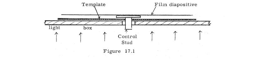
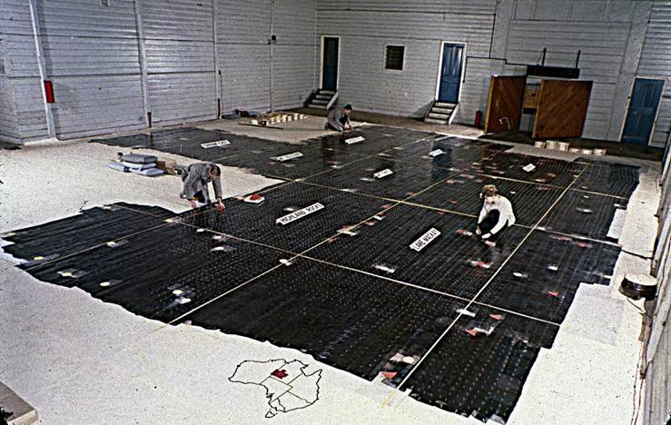
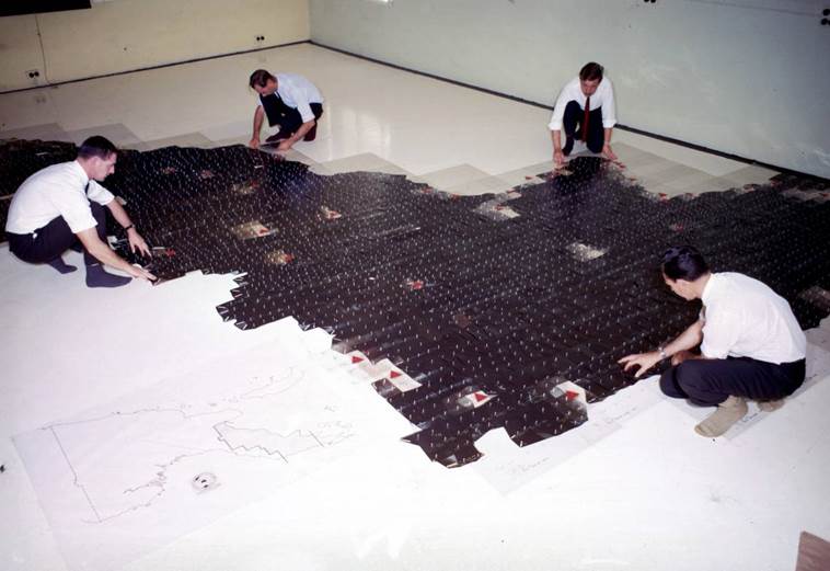
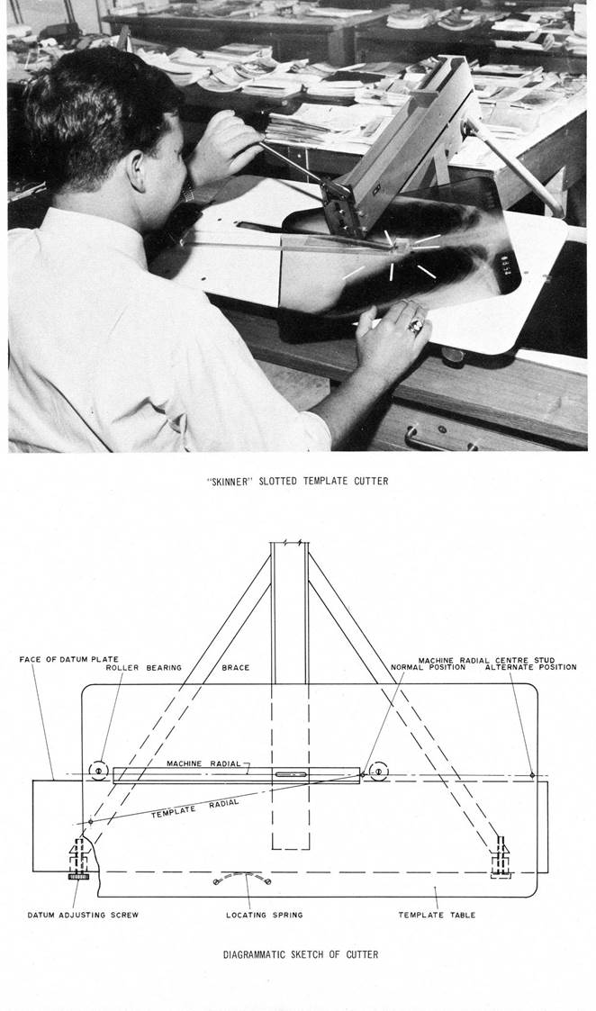
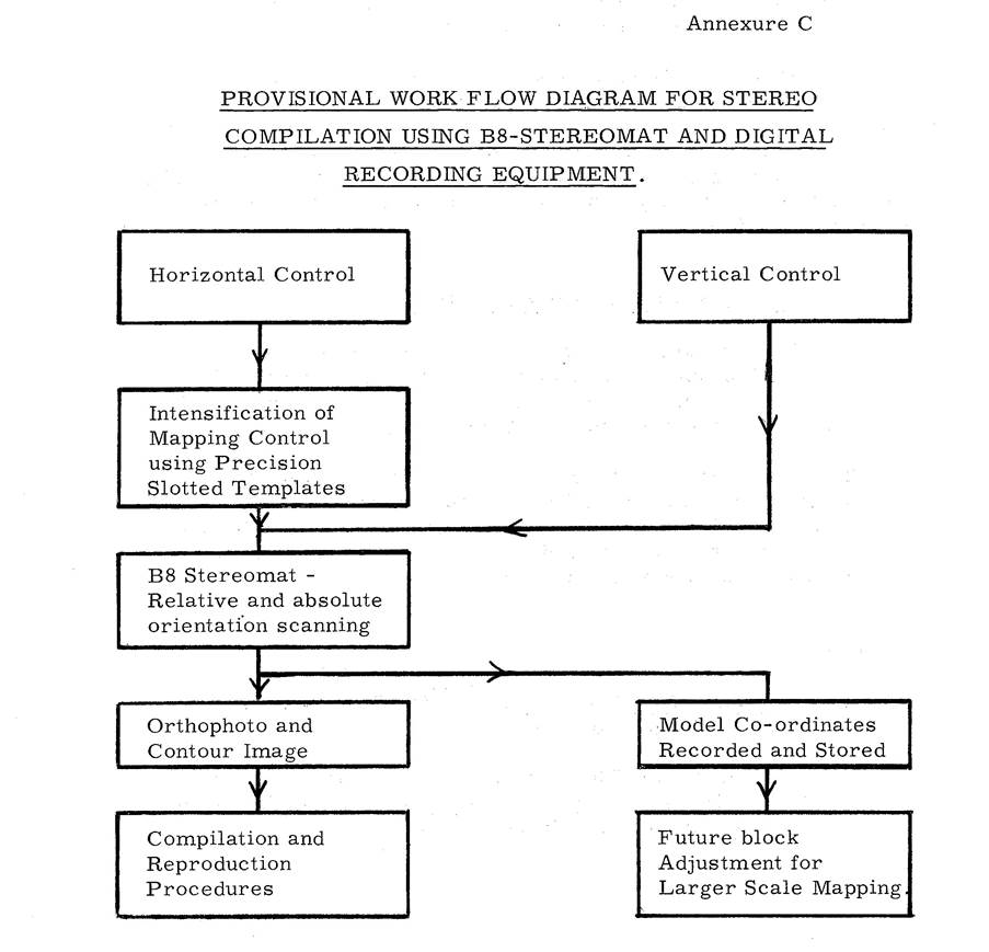
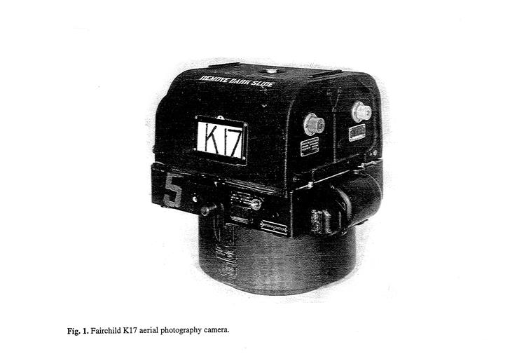
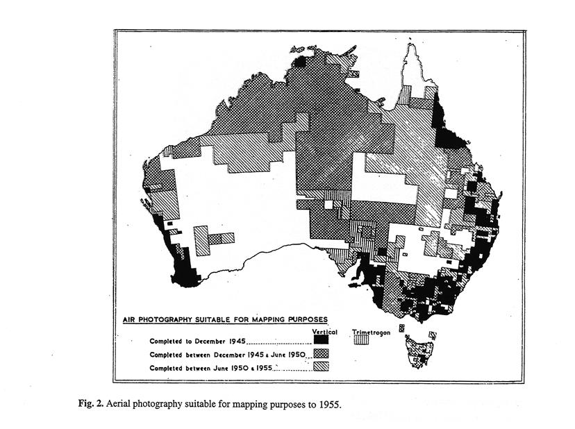
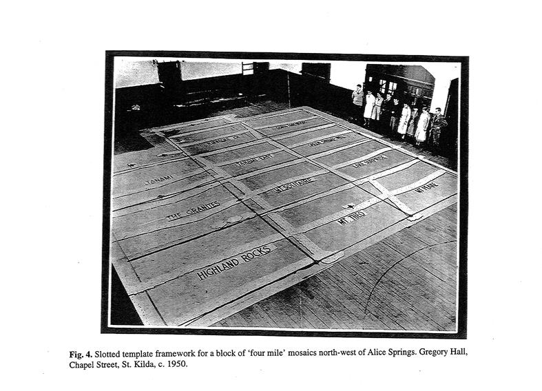
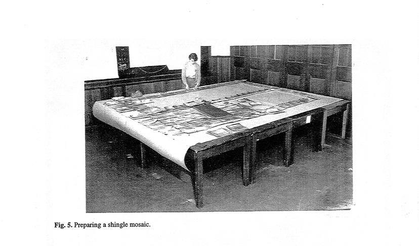
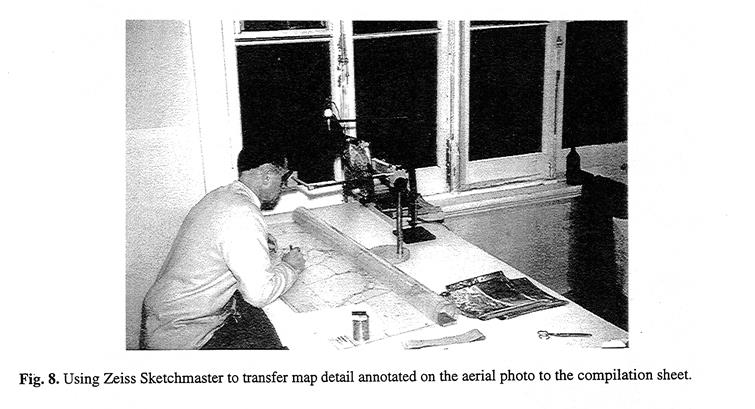
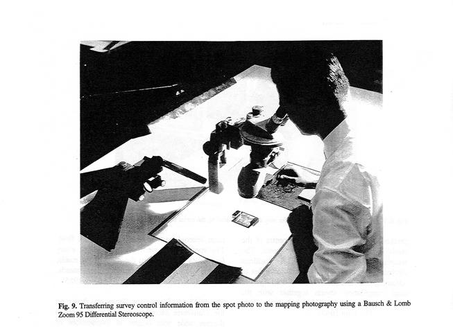
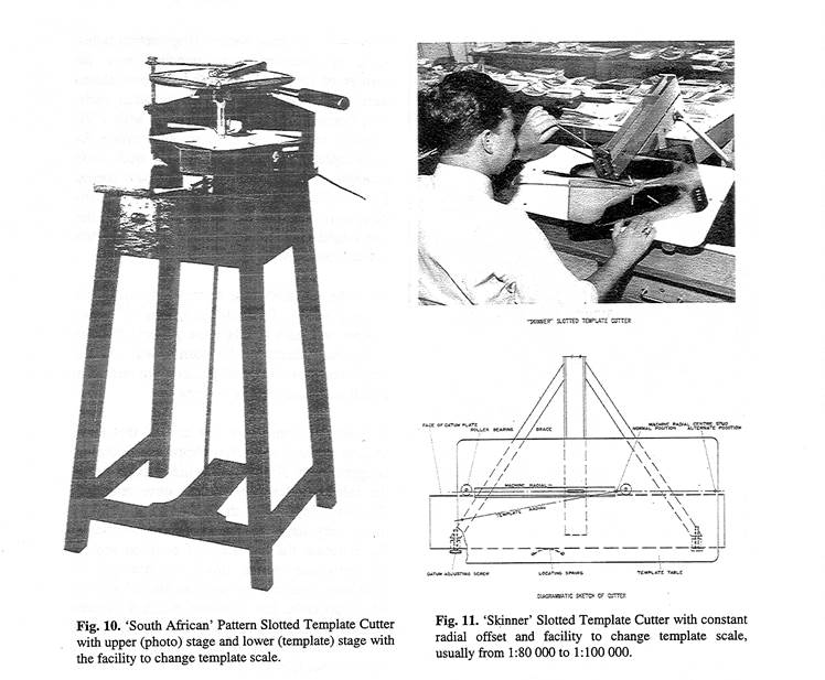
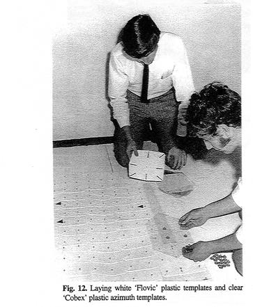
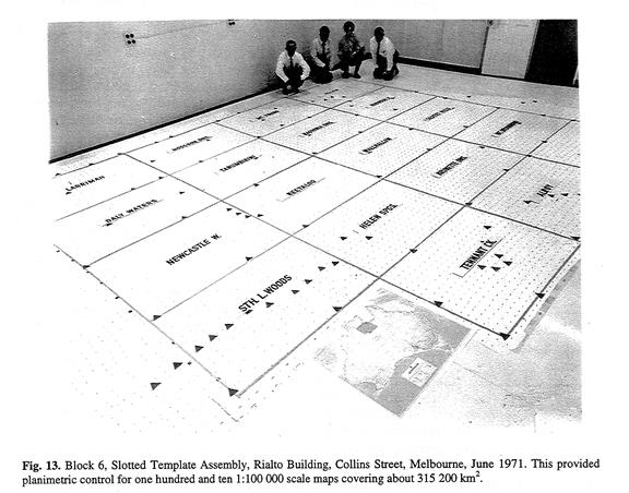
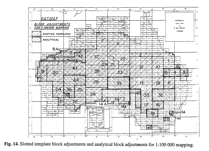
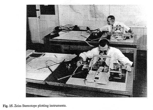
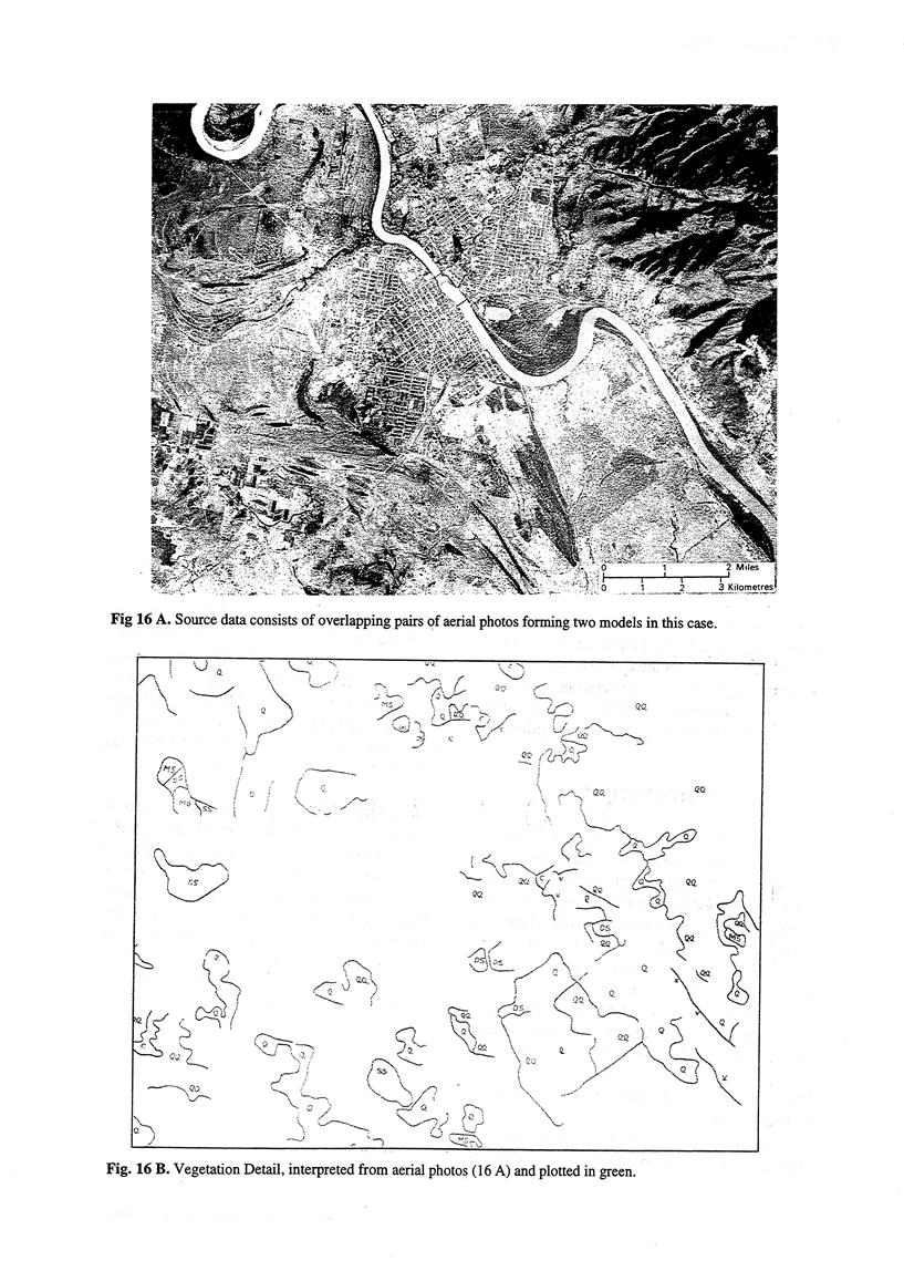
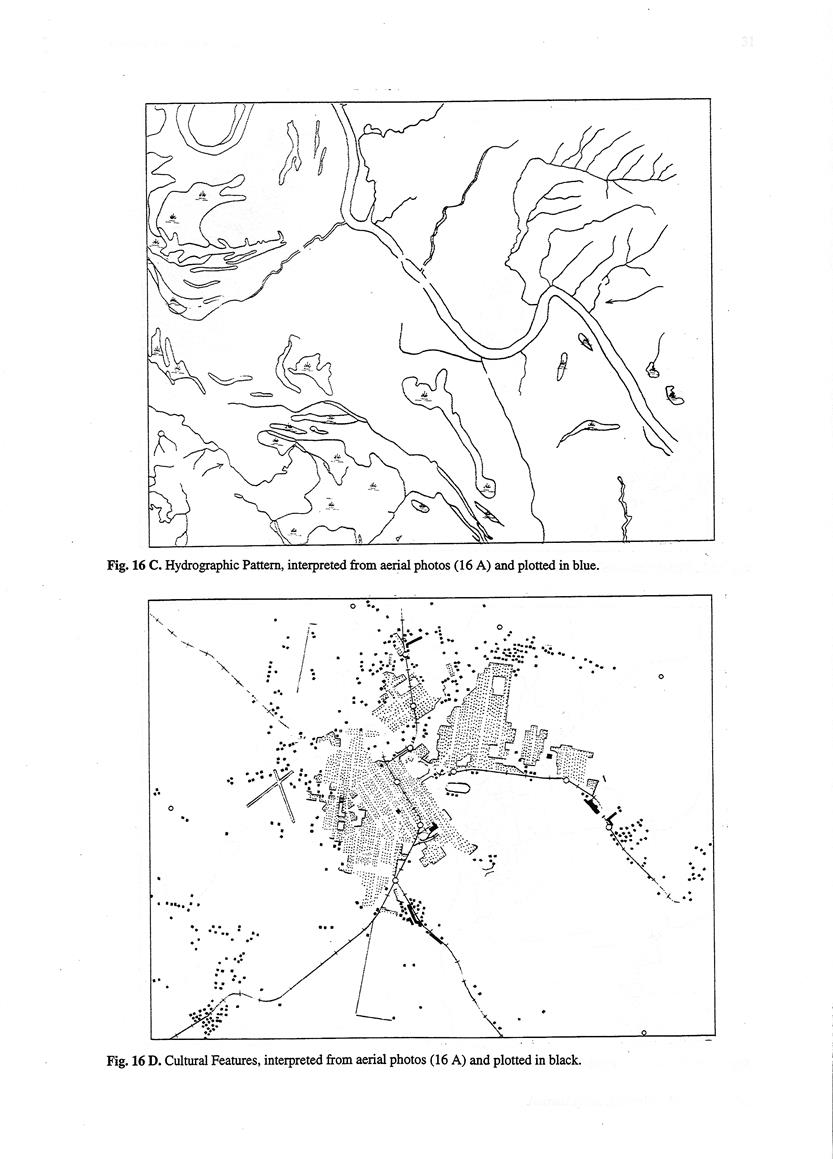
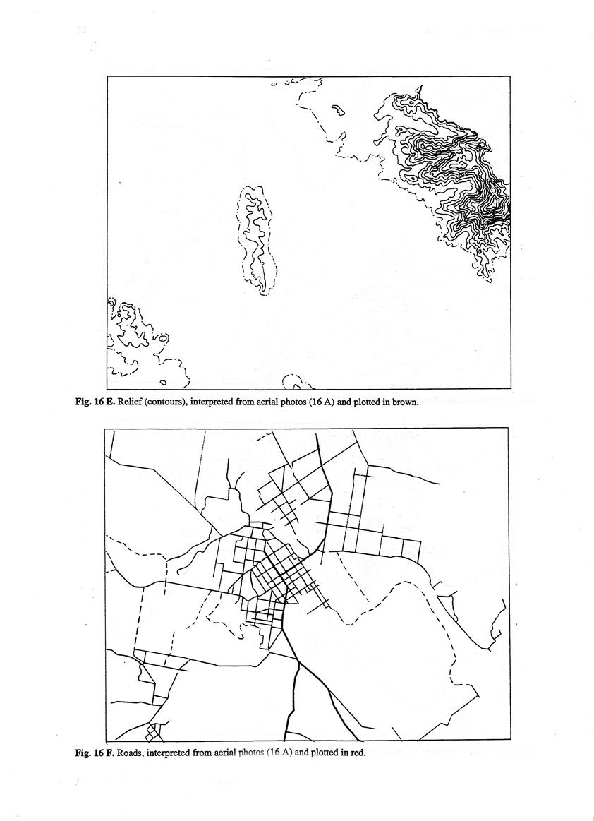
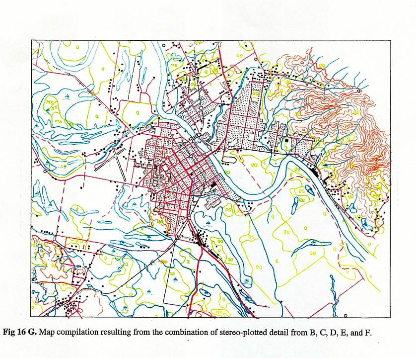
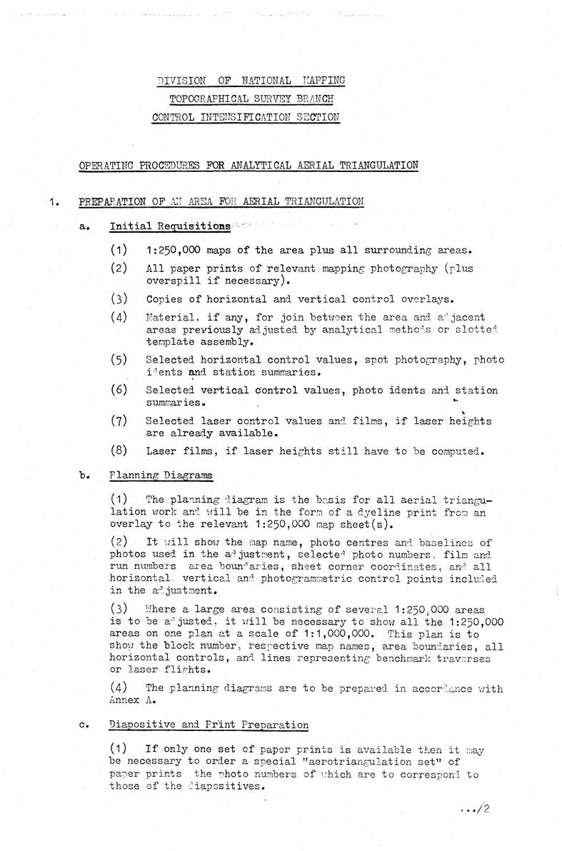
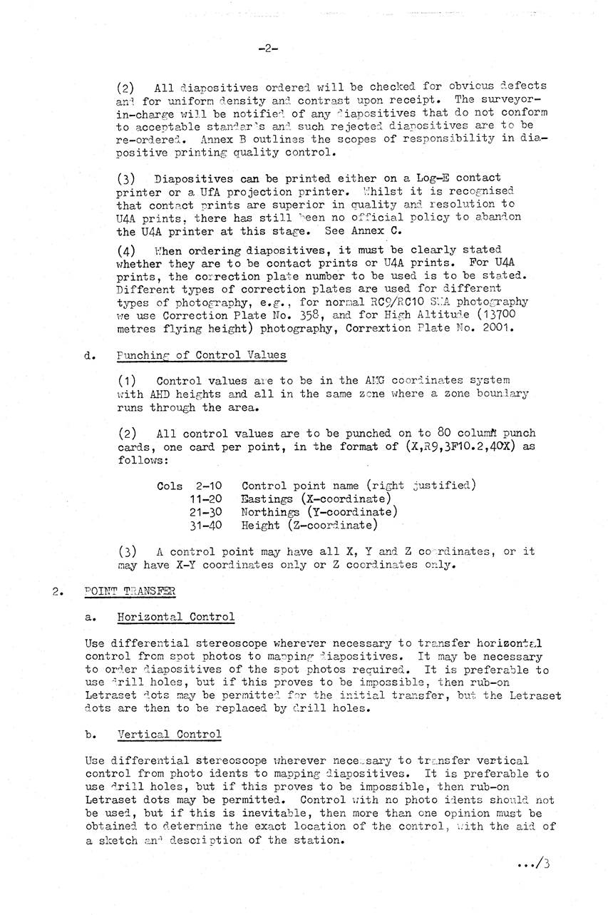
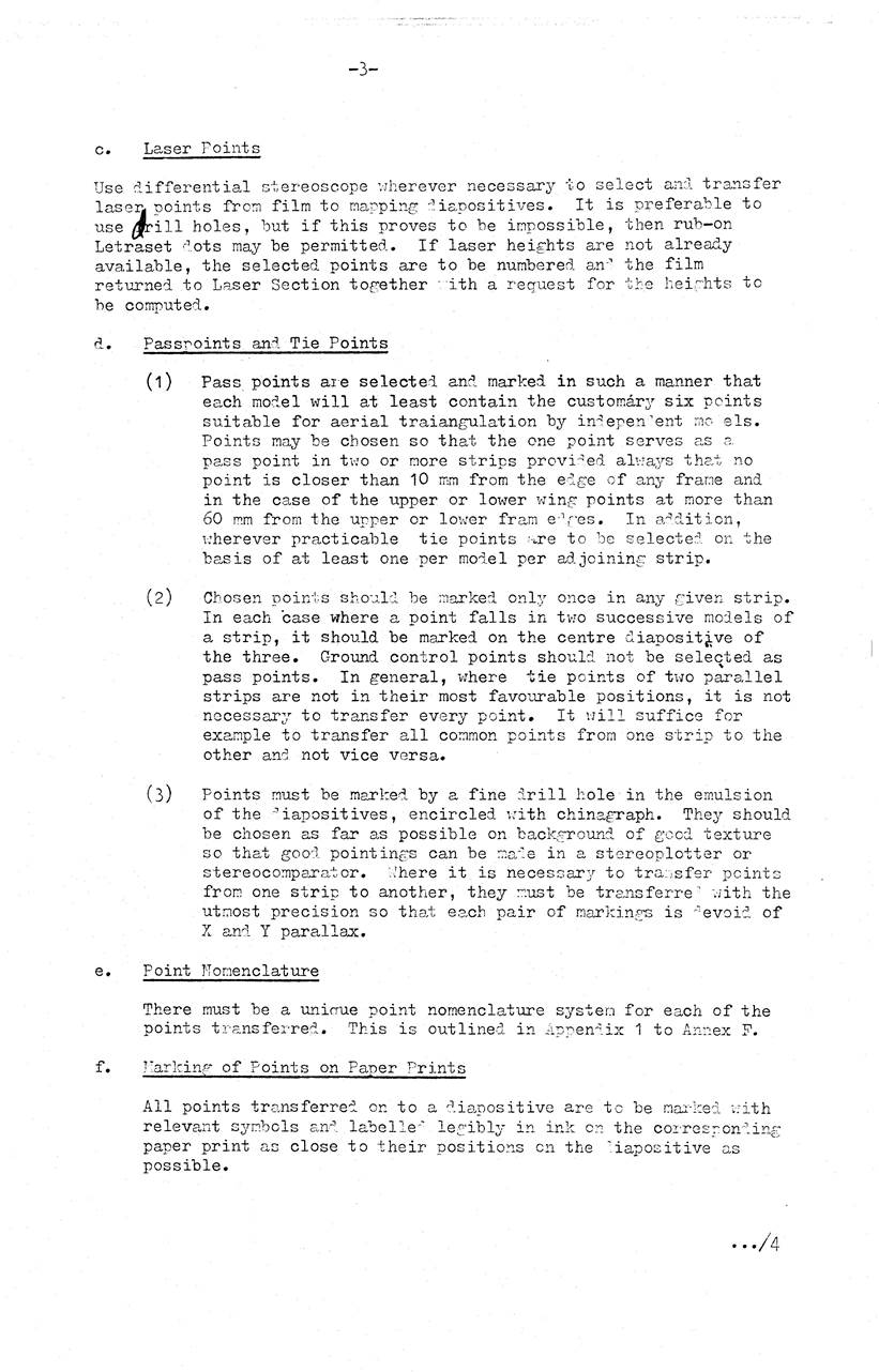
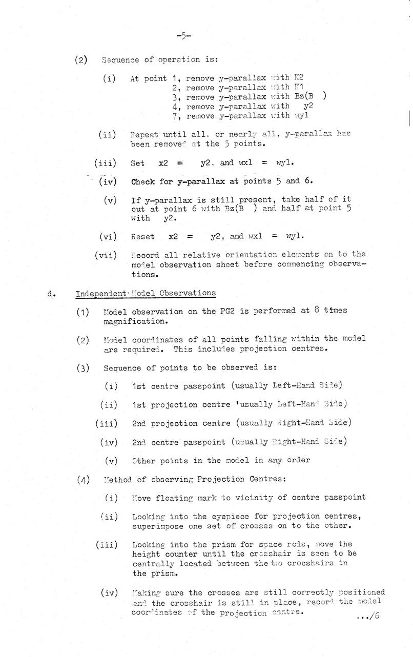
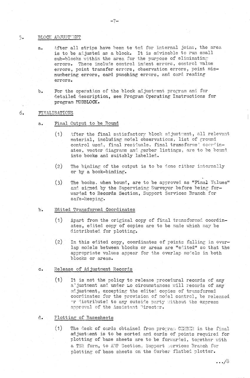
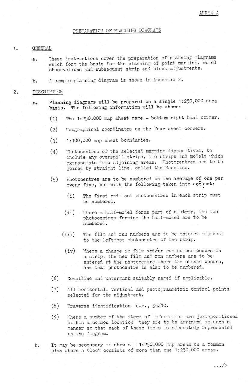
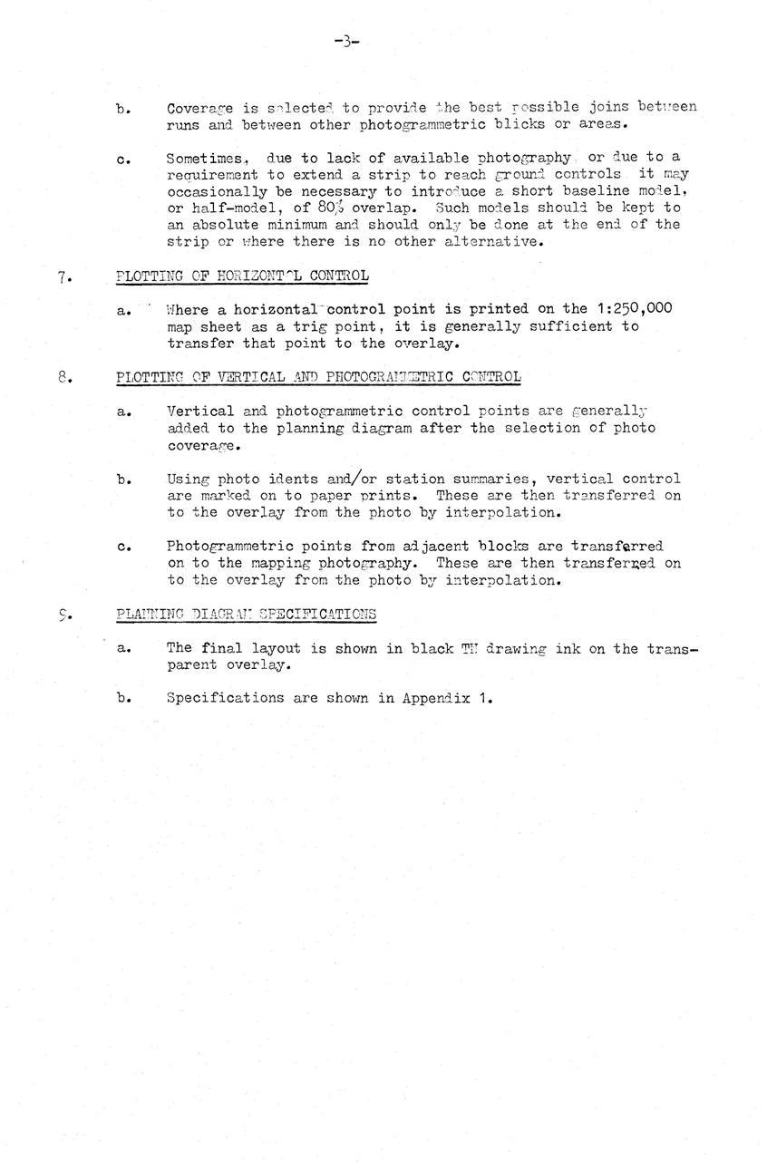
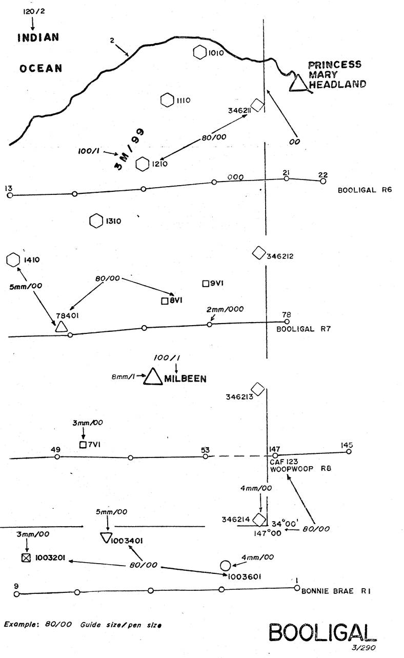
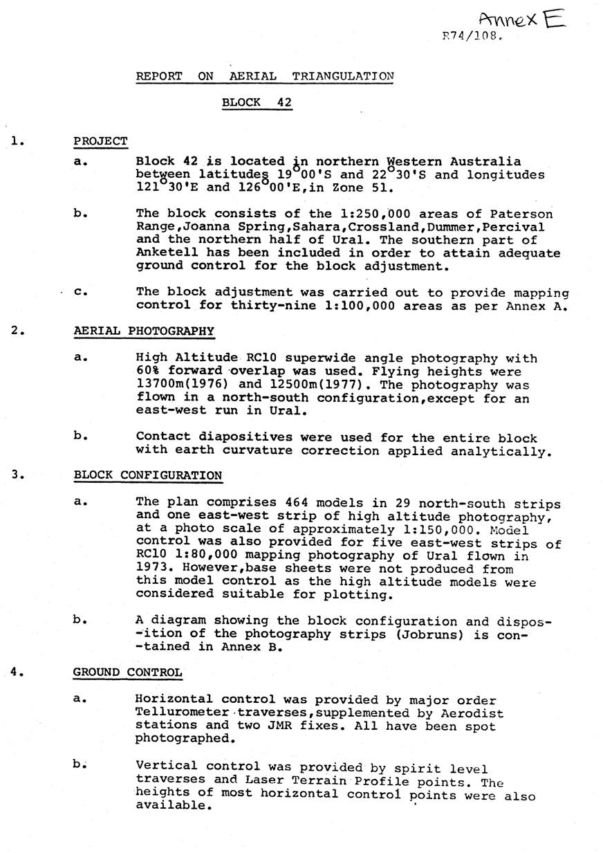
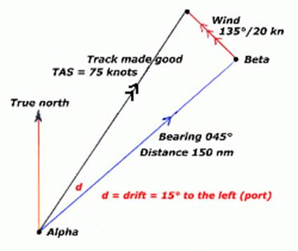
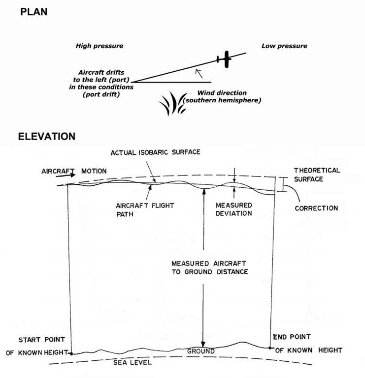
servo traverses the wedge across the slit to compensate for film speed changes
as dictated by different V/H values. The servo also maintains a constant film
illumination under varying ambient light conditions.
the film but a nominal gap exists between film and plate to eliminate continuous
rubbing.